QualityThought Learn ML – Code
JULY 31 2022: SQL Programming
SELect * from olym.olym_events

select * from olym.olym_base_events

select * from olym.olym_disciplines

select ID, SPORT from olym.olym_sports

select S.ID, S.SPORT, D.Discipline from olym.olym_sports S, olym.olym_disciplines D,   WHERE s.ID = d.sport_id

select * from olym.olym_medals_view where Edition=1996 and discipline='Tennis' and Gender='Men' and event = 'singles'
select * from olym.olym_medals_view where Edition>1950 and NOC='IND' and athlete like '%KU%' order by edition desc
Date: AUGUST 1 2022
import sqlite3
import pymysql
con = sqlite3.connect('library.db')  #1. Make connection to your Database
#con = pymysql()
dbobj = con.cursor()
command = '''
Create Table Books(
BOOKID INTEGER PRIMARY KEY,
TITLE TEXT,
PRICE REAL,
COPIES INTEGER
)
'''
command = '''
Insert Into BOOKS(
BookID, Title, Price,Copies
) values(3, 'Practice Machine Learning',410.25, 18)
'''
#dbobj.execute(command)
#con.commit()

command = '''
Delete from Books where Bookid=2
'''
#dbobj.execute(command)
#con.commit()

command = '''
Update Books set copies = 9 where Bookid=3
'''
#dbobj.execute(command)
command = '''
Select * from Books
'''
dbobj.execute(command)
records = dbobj.fetchall()
for r in records:
    current_count = r[3]
    print(r[3])  #Tuple

if current_count >0:
    command = '''
    Update Books set copies = '%d' where Bookid=3
    '''%(current_count-1)
    dbobj.execute(command)
    con.commit()
else:
    print("Sorry, we do not have any copies left")
print("After removing one value: ")
command = '''
Select * from Books where BookID=3
'''
dbobj.execute(command)
records = dbobj.fetchall()
for r in records:
    #current_count = r[3]
    print(r)
    #print(r[3])  #Tuple

while True:
    print("1. Add a New Book")
    print("2. Issue a Book")
    print("3. Display all books")
    print("4. Return a book")
    print("5. Exit")
    ch=int(input("Enter your choice: "))
AUGUST 2 2022
# File operations:
## Read - r  /  r+
## Write - w   /  w+
## Append - a
fileobj = open("files\\myfile.txt","a")
my_poem = '''HI
How are you today
You should be fine today
lets have a great day today
Enjoy your day today'''
print(fileobj.writable())
fileobj.write(my_poem)
fileobj.close()
fileobj = open("files\\myfile.txt","r")
output = fileobj.read(100)
fileobj.seek(0)
print(output)
output = fileobj.readline()
#output = fileobj.readlines()
print(output)
print("---------------")
fileobj.seek(49)
output = fileobj.read(10)
print(output)
fileobj.close()
## Read and remove vowels and save back
# File operations:
## Read - r  /  r+
## Write - w   /  w+
## Append - a
fileobj = open("files\\myfile.txt","w")
my_poem = '''HI
How are you today
You should be fine today
lets have a great day today
Enjoy your day today'''
fileobj.write(my_poem)
fileobj.close()
fileobj = open("files\\myfile.txt","r")
output = fileobj.read()
fileobj.close()
for i in "aeiouAEIOU":
    new_content = output.split(i)
    output = "".join(new_content)
fileobj = open("files\\myfile.txt","w")
fileobj.write(output)
fileobj.close()
#JSON

{
    "Name": "Sachin Tendulkar",
    "Teams": ['Mumbai','MI','India'],
    "Kids": {
        "Name": ['Arjun', 'Saara'],
        "Age": [23,25]
    }
}

#load /loads = read from json file
#dump /dumps = to write to json file
import json
txt = '{    "Name": "Sachin Tendulkar",     "Teams": ["Mumbai","MI","India"] , "Branch":["A","B","C"]   }'

jsonobj = json.loads(txt)

print(json.dumps(jsonobj, indent=5, sort_keys=True))
jsonfile = open("myjson.json","w")
json.dump(jsonobj, jsonfile,indent=5)

#Program to read a dictionary using loop and save the content as json in a file

txt = '{"name":"Rohit","teams":["MI","IND","M"]}'
f = open("files\\jsonfile.txt",'w')
json.dump(txt, f,indent=5)
f.close()
f = open("files\\jsonfile.txt",'r')
content = json.load(f)
print("After loading \n",content)
# File operations:
## Read - r  /  r+
## Write - w   /  w+
## Append - a
fileobj = open("files\\myfile.txt","w")
my_poem = '''HI
How are you today
You should be fine today
lets have a great day today
Enjoy your day today'''
fileobj.write(my_poem)
fileobj.close()
fileobj = open("files\\myfile.txt","r")
output = fileobj.read()
fileobj.close()
for i in "aeiouAEIOU":
    new_content = output.split(i)
    output = "".join(new_content)
fileobj = open("files\\myfile.txt","w")
fileobj.write(output)
fileobj.close()
AUGUST 4, 2022
try:
    num = int(input("Enter a number: "))
    a = 5
    b = 0
    val = a / b

except ValueError:
    print("Ending the execution of program because you have not entered a valid number")
except ZeroDivisionError:
    print("Zero division error, please retry")
except Exception:
    print("Not sure what but some error occurred")
finally:
    print("I am in finally")
print("Thank you")

# Errors:
#1. Syntax error
#2. Logical error
#3. Exception or runtime
#4. Exceptions: ZeroDivisionError, ValueError

while True:
    try:
        num1 = int(input("Enter first number: "))
        break
    except ValueError:
        print("Unknown error occurred, please try again")

while True:
    try:
        num2 = int(input("Enter second number: "))
        break
    except ValueError:
        print("Unknown error occurred, please try again")

sum = num1 + num2
print("Total: ",sum)


#WAP to input marks in 5 subjects and calculate total and average- use exception where necessary
class NegativeNumber(BaseException):
    pass
try:
    num_marks = int(input("Total number of subjects: "))
    if num_marks <0:
        raise NegativeNumber
    sum = 0
    for i in range(num_marks):
        while True:
            try:
                marks = int(input("Enter marks in subject " + str(i + 1) + ": "))
                break
            except ValueError:
                print("Invalid marks, try again!")
        sum += marks
    avg = sum / num_marks
    print("Total avg = ", avg)
except ValueError:
    print("Invalid input, exiting...")
except NegativeNumber:
    print("Sorry you are not allowed to enter Negative numbers, exiting...")
6 AUGUST 2022
#lambda function
#anonymous function
l1 = lambda x,y : x*y
print(l1(5,4))

#map:
ls1 = [2,4,8,16,32,64]
ls2=[]
for i in ls1:
    ls2.append(i**2)
print(ls2)

#map in list
result = map(lambda x: x**2, ls1)
print(list(result))

#filter
ls3 = [2,4,6,8,10,12,15,18,20,25,28,30,40]
#I want multiples of 5- that means
#filter out those which are not multiples of five
filtered_val = list(filter(lambda x: x%5==0,ls3))
print(filtered_val)
filtered_val = list(filter(lambda x: x>=18,ls3))
print(filtered_val)

#reduce
ls3 = [2,4,6,8,10,12,15,18,20,25,28,30,40]
#cumulative sum:
sum=0
for i in ls3:
    sum+=i
print("Sum: ",sum)

from functools import reduce
sol = reduce(lambda x,y: x+y, ls3)
print(sol)

# take a list of values (c) and using map convert them into F

#take a list of values and filter out values which are multiples of 3 and 7 only

# take a list of values (c) and using map convert them into F
ls1 = [2,3,54,6,7,87,65]
print(list(map(lambda x : (x*(9/5)+32),ls1)))

#take a list of values and filter out values which are multiples of 3 and 7 only
ls2 = [3,6,21,34,42,63,65,78,189]
print(list(filter(lambda x : x%3==0 and x%7==0,ls2)))
8 AUGUST 2022
Program to read content from wikipedia page:
import requests
link = "https://en.wikipedia.org/wiki/List_of_Indian_people_by_net_worth"
website_content = requests.get(url=link).text
#print(website_content)
from bs4 import BeautifulSoup
s = BeautifulSoup(website_content,'lxml')
#print(s.prettify())
print(s.title.string)
#tables = s.find_all('table')
my_table = s.find('table', class_ = "wikitable sortable")
table_links = my_table.find_all('a')
#print(table_links)
rich_indians =[]
for l in table_links:
    rich_indians.append(l.get('title'))
rich_indians.pop(0)
rich_indians.pop(0)
print(rich_indians)
9 AUGUST 2022
#NUMPY - matrix like datastructure
import numpy as np
x = range(9)
print(type(x))
x = np.reshape(x,(3,3))
print(x)
print(type(x))
print("Shape of the numpy: ",x.shape)
y=[[2,3,4],[5,6,2],[3,7,4]]
y = np.array(y)
print(y)
print(y[0])
print(y[0,2])
print(y[:,2])

#dummy values to the numpy
z = np.zeros((4,4))
print(z)
z = np.ones((4,4))
print(z)
z = np.full((4,4),2)
print(z)
idm1 = np.identity(3, dtype=int)
print(idm1)
print("Operation")
x=[[5,1,0],[1,1,2],[3,0,4]]
x = np.array(x)
y=[[2,3,4],[5,6,2],[3,7,4]]
y = np.array(y)
print(x)
print(y)
#print(x+y)
#print(x-y)
#print(x*y)
print(x/y)
#for above operations both matrices should have same shape
#MATRIX MULTIPLICATION
## condition a *b  matmul m * n => b should be equal to m
x=[[5,1,0],[1,1,2],[3,0,4]]
x = np.array(x)
y=[[2,3,4],[5,6,2],[3,7,4]]
y = np.array(y)
print(x)
print(y)
z = np.matmul(x,y)
print(z)

#determinant
a= np.array([[23,14],[37,28]])
det_a = np.linalg.det(a)
print(det_a)
inv_b = np.linalg.inv(a)
print(inv_b)
print(np.matmul(a,inv_b))

a= np.array([[23,28],[23,28]])
det_a = np.linalg.det(a)
print(det_a)
#Matrix with zero determinant, is singular matrix
inv_b = np.linalg.inv(a)
print(inv_b)
print(np.matmul(a,inv_b))
10 AUGUST 2022
# 3x +4y - 7z = 2
# -2x +y -z = -6
# x +y + z = 2
#form 3 matrices:
## Coefficient matrix
## Variable matrix
## Constant matrix
### Coefficient matrix X Variable Matrix = Constant Matrix
# 5X = 15  => X = 15/5
# => variable matrx = inverse of Coefficient matrix * Constant matrix
import numpy as np
coeff_matrix = np.array([[3,4,-7],[-2,1,-1],[1,1,1]])
cont_matrix = np.array([[2],[-6],[2]])
det_coeff = np.linalg.det(coeff_matrix)
if det_coeff==0:
    print("Solution is not possible")
else:
    variable_mat = np.matmul(np.linalg.inv(coeff_matrix) , cont_matrix)
    print(variable_mat)
AUGUST 11, 2022
# Permutation & Combination
# => selecting r things from n things
 ##  in Permutation Order Matters - 2 cases: with or without replacement
 ## in Combination Order Doesnt Matter - 2 cases: with or without replacement

 ### P = n! / (n-r)!
 ### C = n! / [(n-r)!  r!]

 # 10 students - 4students->

 #4 Coats, 3 hats, 2 umbrellas

from scipy.special import perm,comb
result = comb(10,4)
print(result)
# 6B , 4 G => 4 Students:
#1. 4B+0G, 3B +1G, 2B + 2G, 1B + 3G, 0B+4G
c1 = comb(6,4,repetition=True)
c2 = comb(6,3) + comb(4,1)
c3 = comb(6,2) + comb(4,2)
c4 = comb(6,1) + comb(4,3)
c5 = comb(4,4)
result = c1+c2+c3+c4+c5
print(result)

##4 Coats, 3 hats, 2 umbrellas
## 2
c1=perm(4,2)
c2 = perm(3,2)
c3 = perm(2,2)
result = c1 * c2 * c3
print(result)

###################
#Own a factory: 2 kinds of products: desktop & laptops
#each desktop gives you Rs 1000
# each laptop gives you Rs 2000
### How much is your profit?
# profit: 1000 * D  +  2000 * L  =========> OBJECTIVE
# manpower: 5000 min: D= 100 L= 41
##50 min     120 min <= Total of 5000 min
##1    2   <= 1000
# D = 1000 , L=500

##HDD: 1000
# 1 1:

# F -Full worker, P , R
#Obj:  200*F + 80 * P + 40*R
#Constraints:
## 200*F + 80 * P + 40*R <=4000
14 AUGUST 2022
## Scipy
import numpy as np
from scipy.optimize import minimize, LinearConstraint, linprog

x = 1;y = 1
profit_desktop, profit_notebook = 1000, 750
profit = profit_desktop*x + profit_notebook*y

obj_function = [-profit_notebook, -profit_desktop] #converting maximize to minimize
## constraints
lhs_contraint = [[1,1],[1,2],[4,3]]
rhs_constraint = [10000,15000,25000]
bounds =[(0,float("inf")),
         (0,10000)]
opt_sol = linprog(c=obj_function, A_ub=lhs_contraint, b_ub=rhs_constraint,bounds=bounds,
                  method="revised simplex")
if opt_sol.success:
    print("Solution is ",opt_sol)

# x + y +2000 =10000
# x+2y +0 =15000  #
# 4x + 3y + 0 <= 25000 #
# 1000 7000


### Pandas: library
### data type is called dataframe
data = [[1,"Rohit"],[2,"Pant"],[3,"Surya"],[4,"Dhawan"],[5,"Kohli"]]
import pandas as pd
data_df = pd.DataFrame(data, columns=["Position","Player"],index=["First","Second","Third","Forth","Fifth"])
print(data_df)

#fruit production
data = {
    "Apples": [100,200,150,250],
    "Oranges":[250,200,300,200],
    "Mangoes":[150,700,800,50]
}
data_df = pd.DataFrame(data,index=["Q1 2021","Q2 2021","Q3 2021","Q4 2021"])
print(data_df)
16 AUGUST 2022
# Monday to Friday - 10am to 12 noon
# online class

## Saturday - only offline class- practice
## Sunday - only - practice
##    #######################
#Pandas
import pandas as pd
link="https://raw.githubusercontent.com/swapnilsaurav/Dataset/master/hotel_bookings.csv"
hotel_df = pd.read_csv(link)
#print(hotel_df)
df_shape = hotel_df.shape
print("Shape: ",df_shape)
print("Total rows = ",df_shape[0])
print("Data types: ", hotel_df.dtypes)
print(hotel_df['hotel'])
#filter numeric column
import numpy as np
numericval_df = hotel_df.select_dtypes(include=[np.number])
print(numericval_df)
numeric_cols =numericval_df.columns.values
print("Numeric columns in Hotel df is \n",numeric_cols)
#get non-numeric values
#exclude
nonnumericval_df = hotel_df.select_dtypes(exclude=[np.number])
print(nonnumericval_df)
nonnumeric_cols =nonnumericval_df.columns.values
print("Numeric non-columns in Hotel df is \n",nonnumeric_cols)

import matplotlib.pyplot as plt
#from matplotlib.pyplot import figure
#plt.figure((6,3))
import seaborn as sns
cols_25 = hotel_df.columns[:25]
colors = ['#FF5733','#3333FF']
sns.heatmap(hotel_df[cols_25].isnull(), cmap=sns.color_palette(colors))
plt.show()

for c in hotel_df.columns:
    pct_missing = (np.mean(hotel_df[c].isnull()))*100
    if pct_missing>85:
        print(f"{c} - {pct_missing}%")
17 AUGUST 2022
#Pandas
import pandas as pd
link="https://raw.githubusercontent.com/swapnilsaurav/Dataset/master/hotel_bookings.csv"
hotel_df = pd.read_csv(link)
#print(hotel_df)
df_shape = hotel_df.shape
#print("Shape: ",df_shape)
#print("Total rows = ",df_shape[0])
#print("Data types: ", hotel_df.dtypes)
#print(hotel_df['hotel'])
#filter numeric column
import numpy as np
numericval_df = hotel_df.select_dtypes(include=[np.number])
print(numericval_df)
numeric_cols =numericval_df.columns.values
print("Numeric columns in Hotel df is \n",numeric_cols)
#get non-numeric values
#exclude
nonnumericval_df = hotel_df.select_dtypes(exclude=[np.number])
print(nonnumericval_df)
nonnumeric_cols =nonnumericval_df.columns.values
#print("Numeric non-columns in Hotel df is \n",nonnumeric_cols)

import matplotlib.pyplot as plt
#from matplotlib.pyplot import figure
#plt.figure((6,3))
import seaborn as sns
cols_25 = hotel_df.columns[:25]
colors = ['#FF5733','#3333FF']
sns.heatmap(hotel_df[cols_25].isnull(), cmap=sns.color_palette(colors))
plt.show()

for c in hotel_df.columns:
    missing = hotel_df[c].isnull()
    num_missing = np.sum(missing)

    pct_missing = (np.mean(hotel_df[c].isnull())) * 100
    if pct_missing > 85:
        print(f"{c} - {pct_missing}%")

for c in hotel_df.columns:
    missing = hotel_df[c].isnull()
    num_missing = np.sum(missing)
    if num_missing >0:
        hotel_df[f'{c}_missing'] = missing
#print(hotel_df.shape)
#create missing total column
missing_col_list = [c for c in hotel_df.columns if '_missing' in c]
print(missing_col_list)
hotel_df['_missing'] = hotel_df[missing_col_list].sum(axis=1)
#create bar graph
hotel_df['_missing'].value_counts().reset_index().plot.bar(x='index',y="_missing")
plt.show()
# delete the not required columns and rows
print("Before row dropping: ",hotel_df.shape)
row_missing = hotel_df[hotel_df['_missing'] > 10].index
print("========== ROW MISSING: \n",row_missing)
hotel_df = hotel_df.drop(row_missing, axis=0)  #axis = 0: look for each row
hotel_df = hotel_df.drop(['company'],axis=1)
print("After row & column dropping: ",hotel_df.shape)

for c in hotel_df.columns:
    missing = hotel_df[c].isnull()
    num_missing = np.sum(missing)

    pct_missing = (np.mean(hotel_df[c].isnull())) * 100
    if pct_missing > 0:
        print(f"{c} - {pct_missing}%")

med = hotel_df['babies'].median()
hotel_df['babies'] = hotel_df['babies'].fillna(med)
med = hotel_df['children'].median()
hotel_df['children'] = hotel_df['children'].fillna(med)

mode = hotel_df['meal'].describe()['top']
hotel_df['meal'] = hotel_df['meal'].fillna(mode)

mode = hotel_df['country'].describe()['top']
hotel_df['country'] = hotel_df['country'].fillna(mode)

med = hotel_df['agent'].median()
hotel_df['agent'] = hotel_df['agent'].fillna(med)

mode = hotel_df['deposit_type'].describe()['top']
hotel_df['deposit_type'] = hotel_df['deposit_type'].fillna(mode)

print("Missing values after all replacement:")
for c in hotel_df.columns:
    missing = hotel_df[c].isnull()
    num_missing = np.sum(missing)

    pct_missing = (np.mean(hotel_df[c].isnull())) * 100
    if pct_missing > 0:
        print(f"{c} - {pct_missing}%")
22 AUGUST 2022
24 AUGUST 2022
AUGUST 25 2022 (Machine Learning)
29 AUGUST 2022
import pandas as pd
txt_df = pd.read_csv("https://raw.githubusercontent.com/swapnilsaurav/OnlineRetail/master/order_reviews.csv")

#NLP: Natural Language Processing - NLP Analysis
#1. entire text to lowercase
#2. non-english, decomposition - convert non-english characters into English
#3. converting utf8
#4. Tokensize: converting sentence into words
#5. Removal Stop words - words which doesnt carry meaning
######################
import unicodedata
import nltk
#nltk.download('punkt')
#nltk.download('stopwords')

#function to normalize text
def normalize_text(word):
    return unicodedata.normalize('NFKD',word).encode('ascii', errors = 'ignore').decode('utf-8')
#get stop words database
STOP_WORDS = set(normalize_text(word) for word in nltk.corpus.stopwords.words('portuguese'))
#STOP_WORDS =

## function tp perform all the analysis
def convert_into_lowercase(comments):
    lower_case = comments.lower()
    unicode = unicodedata.normalize('NFKD',lower_case).encode('ascii', errors = 'ignore').decode('utf-8')
    words = nltk.tokenize.word_tokenize(unicode)
    words = tuple(word for word in words if word not in STOP_WORDS and word.isalpha())
    return words

analysis_txt = txt_df[txt_df['review_comment_message'].notnull()].copy()
#print(analysis_txt['review_comment_message'])
analysis_txt['review_txt'] =analysis_txt['review_comment_message'].apply(convert_into_lowercase)
#print(analysis_txt['review_txt'])


# Dont buy now
# unigram => Dont, buy, now
# bigram=> Dont buy, buy now
# trigram => Dont buy now

# create 2 datasets
rating_5 = analysis_txt[analysis_txt['review_score']==5]
rating_1 = analysis_txt[analysis_txt['review_score']==1]

def word_to_grams(words):
    unigrams,bigrams,trigrams = [],[],[]
    for w in words:
        unigrams.extend(w)
        bigrams.extend(" ".join(bigram) for bigram in nltk.bigrams(w))
        trigrams.extend(" ".join(trigram) for trigram in nltk.trigrams(w))
    return unigrams,bigrams,trigrams

unigram_5,bigram_5,trigram_5 = word_to_grams(rating_5['review_txt'])
unigram_1,bigram_1,trigram_1 = word_to_grams(rating_1['review_txt'])

#print(unigram_1)
#input()
#print(bigram_1)
#input()
print(trigram_1)
#input()
Z Score and Emphirical Rule (click here to access)
SEPTEMBER 9, 2022 CLASS NOTES
import pandas as pd
import numpy as np
data_df = pd.read_csv("https://raw.githubusercontent.com/swapnilsaurav/MachineLearning/master/3_Startups.csv")
X = data_df.iloc[:,:-1].values
y = data_df.iloc[:,-1].values
from sklearn.preprocessing import LabelEncoder, OneHotEncoder
le_obj = LabelEncoder()
X[:,3] = le_obj.fit_transform(X[:,3])
from sklearn.compose import ColumnTransformer
transform = ColumnTransformer([('one_hot_encoder',OneHotEncoder(),[3])],remainder='passthrough')
X=np.array(transform.fit_transform(X), dtype=np.float)
################### ABOVE THIS COMMON FOR ALL
#drop one column
X = X[:,1:]
#print(X)
from sklearn.model_selection import train_test_split
X_train, X_test, y_train, y_test = train_test_split(X,y, test_size=0.25)
############################## REGRESSION OR CLASSIFICATION
from sklearn.linear_model import LinearRegression
regressor = LinearRegression()
### POLYNOMIAL REGRESSION
from sklearn.preprocessing import PolynomialFeatures
from sklearn.pipeline import Pipeline
parameter = [('polynomial',PolynomialFeatures(degree=2)),('modal',LinearRegression())]
Pipe = Pipeline(parameter)
Pipe.fit(X,y)
from sklearn import metrics
y_prep_poly = Pipe.predict(X_test)
mse = metrics.mean_squared_error(y_test,y_prep_poly)
rmse = np.sqrt(mse)
r2 = metrics.r2_score(y_test,y_prep_poly)
print("POLYNOMIAL: R2 and RMSE: ", r2,rmse)
########### BELOW IS COMMON FOR ALL REGRESSION
regressor.fit(X_train, y_train)
y_pred = regressor.predict(X_test)
from sklearn.svm import SVR
svr_obj = SVR(kernel='linear')
svr_obj = SVR(kernel='poly',degree=3, C=100)
mse = metrics.mean_squared_error(y_test,y_pred)
rmse = np.sqrt(mse)
r2 = metrics.r2_score(y_test,y_pred)
print("R2 and RMSE: ", r2,rmse)
import statsmodels.api as sm
from statsmodels.api import OLS
X = sm.add_constant(X)
summary = OLS(y,X).fit().summary()
print(summary)
#First elimination
X_select = X[:,[0,3,5]]
X = sm.add_constant(X)
summary = OLS(y,X_select).fit().summary()
print(summary)
import pandas as pd
import numpy as np
from sklearn import metrics
data_df = pd.read_csv("https://raw.githubusercontent.com/swapnilsaurav/MachineLearning/master/3_Startups.csv")
X = data_df.iloc[:,:-1].values
y = data_df.iloc[:,-1].values

from sklearn.preprocessing import LabelEncoder, OneHotEncoder
le_obj = LabelEncoder()
X[:,3] = le_obj.fit_transform(X[:,3])
from sklearn.compose import ColumnTransformer
transform = ColumnTransformer([('one_hot_encoder',OneHotEncoder(),[3])],remainder='passthrough')
X=np.array(transform.fit_transform(X), dtype=np.float)
################### ABOVE THIS COMMON FOR ALL
#drop one column
X = X[:,1:]
#print(X)
from sklearn.model_selection import train_test_split
X_train, X_test, y_train, y_test = train_test_split(X,y, test_size=0.25)
############################## REGRESSION OR CLASSIFICATION


from sklearn.svm import SVR
svr_obj = SVR(kernel='linear')
svr_obj = SVR(kernel='poly',degree=3, C=100)
i=0.03
while i<=0.06:
    i+=0.005
    for j in range(10,1000,200):
        svr_obj = SVR(kernel='rbf', C=j,gamma=i)
        y_pred = svr_obj.fit(X_train, y_train).predict(X_test)
        mse = metrics.mean_squared_error(y_test,y_pred)
        rmse = np.sqrt(mse)
        r2 = metrics.r2_score(y_test,y_pred)
        print(f"gamma = {i}, C = {j}, RMSE = {rmse} ")

from sklearn.tree import DecisionTreeRegressor
regressor = DecisionTreeRegressor()
regressor.fit(X_train,y_train)
y_pred = regressor.predict(X_test)
se = metrics.mean_squared_error(y_test,y_pred)
rmse = np.sqrt(mse)
r2 = metrics.r2_score(y_test,y_pred)
print(f" RMSE = {rmse} and R2 = {r2} ")

from sklearn.ensemble import RandomForestRegressor
print("Performing Random Forest regressor")
for i in range(50,1000,75):
    regressor = RandomForestRegressor(n_estimators=i)
    regressor.fit(X_train,y_train)
    y_pred = regressor.predict(X_test)
    mse = metrics.mean_squared_error(y_test,y_pred)
    rmse = np.sqrt(mse)
    r2 = metrics.r2_score(y_test,y_pred)
    print(f" RMSE = {rmse} and R2 = {r2} ")

#Ridge LAsso as assignment
SEPTEMBER 11, 2022
import numpy as np
import pandas as pd
dataset = pd.read_csv("https://raw.githubusercontent.com/swapnilsaurav/MachineLearning/master/5_Ads_Success.csv")
X =dataset.iloc[:,1:4].values
y =dataset.iloc[:,4].valuesfrom sklearn.preprocessing import LabelEncoder, OneHotEncoder
from sklearn.compose import ColumnTransformer
label = LabelEncoder()
X[:,0] = label.fit_transform(X[:,0])
transform = ColumnTransformer([('one_hot_encoder',OneHotEncoder(),[0])],remainder='passthrough')
X=np.array(transform.fit_transform(X), dtype=np.float)
X= X[:,1:]
print(X)from sklearn.preprocessing import StandardScaler
sc = StandardScaler()
X = sc.fit_transform(X)from sklearn.model_selection import train_test_split
X_train,X_test,y_train,y_test = train_test_split(X,y, test_size=0.25, random_state=1)
##############################
##classifier
from sklearn.linear_model import LogisticRegression
classifier = LogisticRegression()
classifier.fit(X_train, y_train)
y_pred = classifier.predict(X_test)####################################
#Model Evaluation: build confusion matrix
from sklearn.metrics import classification_report, accuracy_score, confusion_matrix
cm_test = confusion_matrix(y_test, y_pred)
y_train_pred = classifier.predict(X_train)
cm_train = confusion_matrix(y_train, y_train_pred)
accuracy_test = accuracy_score(y_test, y_pred)
accuracy_train = accuracy_score(y_train, y_train_pred)print("CONFUSION MATRIX:\n-------------------")
print("TEST: \n",cm_test)
print("\nTRAINING: \n",cm_train)
print("\n ACCURACY SCORE OF TEST: ",accuracy_test)
print("\nACCURACY SCORE OF TRAINING: ",accuracy_train)#############################
12 SEPTEMBER 2022: CLASSIFICATION – SVC< DECISION TREE
import numpy as np
import pandas as pd
dataset = pd.read_csv("https://raw.githubusercontent.com/swapnilsaurav/MachineLearning/master/5_Ads_Success.csv")
X =dataset.iloc[:,1:4].values
y =dataset.iloc[:,4].values

from sklearn.preprocessing import LabelEncoder, OneHotEncoder
from sklearn.compose import ColumnTransformer
label = LabelEncoder()
X[:,0] = label.fit_transform(X[:,0])
transform = ColumnTransformer([('one_hot_encoder',OneHotEncoder(),[0])],remainder='passthrough')
X=np.array(transform.fit_transform(X), dtype=np.float)
X= X[:,1:]
print(X)

from sklearn.preprocessing import StandardScaler
sc = StandardScaler()
X = sc.fit_transform(X)

from sklearn.model_selection import train_test_split
X_train,X_test,y_train,y_test = train_test_split(X,y, test_size=0.25, random_state=1)
##############################
##classifier
#from sklearn.linear_model import LogisticRegression
#classifier = LogisticRegression()
#from sklearn.svm import SVC
#classifier = SVC(kernel='rbf',gamma=0.1,C=100)
from sklearn.tree import DecisionTreeClassifier
classifier = DecisionTreeClassifier(criterion='entropy')
classifier.fit(X_train, y_train)
y_pred = classifier.predict(X_test)

####################################
#Model Evaluation: build confusion matrix
from sklearn.metrics import classification_report, accuracy_score, confusion_matrix
cm_test = confusion_matrix(y_test, y_pred)
y_train_pred = classifier.predict(X_train)
cm_train = confusion_matrix(y_train, y_train_pred)
accuracy_test = accuracy_score(y_test, y_pred)
accuracy_train = accuracy_score(y_train, y_train_pred)

print("CONFUSION MATRIX:\n-------------------")
print("TEST: \n",cm_test)
print("\nTRAINING: \n",cm_train)
print("\n ACCURACY SCORE OF TEST: ",accuracy_test)
print("\nACCURACY SCORE OF TRAINING: ",accuracy_train)

#############################
# Complete the visualization step
13 SEPTEMBER 2022
import numpy as np
import pandas as pd
dataset = pd.read_csv("https://raw.githubusercontent.com/swapnilsaurav/MachineLearning/master/5_Ads_Success.csv")
X =dataset.iloc[:,1:4].values
y =dataset.iloc[:,4].values

from sklearn.preprocessing import LabelEncoder, OneHotEncoder
from sklearn.compose import ColumnTransformer
label = LabelEncoder()
X[:,0] = label.fit_transform(X[:,0])
transform = ColumnTransformer([('one_hot_encoder',OneHotEncoder(),[0])],remainder='passthrough')
X=np.array(transform.fit_transform(X), dtype=np.float)
X= X[:,1:]
print(X)

from sklearn.preprocessing import StandardScaler
sc = StandardScaler()
X = sc.fit_transform(X)

from sklearn.model_selection import train_test_split
X_train,X_test,y_train,y_test = train_test_split(X,y, test_size=0.25, random_state=1)
##############################
##classifier
from sklearn.ensemble import RandomForestClassifier
#classifier = RandomForestClassifier(n_estimators=100,criterion='entropy')
from sklearn.linear_model import SGDClassifier
classifier = SGDClassifier(max_iter=5000, tol=0.01,penalty="elasticnet")
classifier.fit(X_train, y_train)
y_pred = classifier.predict(X_test)

####################################
#Model Evaluation: build confusion matrix
from sklearn.metrics import classification_report, accuracy_score, confusion_matrix
cm_test = confusion_matrix(y_test, y_pred)
y_train_pred = classifier.predict(X_train)
cm_train = confusion_matrix(y_train, y_train_pred)
accuracy_test = accuracy_score(y_test, y_pred)
accuracy_train = accuracy_score(y_train, y_train_pred)

print("CONFUSION MATRIX:\n-------------------")
print("TEST: \n",cm_test)
print("\nTRAINING: \n",cm_train)
print("\n ACCURACY SCORE OF TEST: ",accuracy_test)
print("\nACCURACY SCORE OF TRAINING: ",accuracy_train)

#############################
# Complete the visualization step
SEPTEMBER 15 2022
Practice project from below link:
1. Predict future sales: https://thecleverprogrammer.com/2022/03/01/future-sales-prediction-with-machine-learning/
2. Predict Tip for the waiter: https://thecleverprogrammer.com/2022/02/01/waiter-tips-prediction-with-machine-learning/
SEPTEMBER 16 2022
1. NLP – Flipkart Review analysis: https://thecleverprogrammer.com/2022/02/15/flipkart-reviews-sentiment-analysis-using-python/
2. Cryptocurrency Price Prediction: https://thecleverprogrammer.com/2021/12/27/cryptocurrency-price-prediction-with-machine-learning/
SEPTEMBER 17 2022
1. Demand Prediction: https://thecleverprogrammer.com/2021/11/22/product-demand-prediction-with-machine-learning/
SEPTEMBER 19 2022
from sklearn.datasets import make_blobs
import matplotlib.pyplot as plt
x,y = make_blobs(n_samples= 300, n_features=2,centers=3, random_state=88)
plt.scatter(x[:,0],x[:,1])
plt.show()
from sklearn.cluster import KMeans
cluster_obj = KMeans(n_clusters=2,init='random',max_iter=500)
Y_val = cluster_obj.fit_predict(x)
print(Y_val)
#plotting the centers
plt.scatter(x[Y_val==0,0],x[Y_val==0,1],c="blue",label="Cluster 0")
plt.scatter(x[Y_val==1,0],x[Y_val==1,1],c="red",label="Cluster 1")
#plt.scatter(x[Y_val==2,0],x[Y_val==2,1],c="black",label="Cluster 2")
#plt.scatter(x[Y_val==3,0],x[Y_val==3,1],c="green",label="Cluster 3")
#plt.scatter(x[Y_val==4,0],x[Y_val==4,1],c="Yellow",label="Cluster 4")
plt.show()
#Measure Distortion for elbow graph
distortion = [] #save distortion from each k value
for i in range(1,50):
    cluster_obj = KMeans(n_clusters=i, init='random', max_iter=500)
    cluster_obj.fit(x)
    distortion.append(cluster_obj.inertia_)
print(distortion)
plt.plot(range(1,50),distortion)
plt.show()


from sklearn.datasets import make_blobs
import matplotlib.pyplot as plt
x,y = make_blobs(n_samples= 20, n_features=2,centers=3, random_state=88)
plt.scatter(x[:,0],x[:,1])
plt.show()
from sklearn.cluster import KMeans
cluster_obj = KMeans(n_clusters=2,init='random',max_iter=500)
Y_val = cluster_obj.fit_predict(x)
print(Y_val)
#plotting the centers
plt.scatter(x[Y_val==0,0],x[Y_val==0,1],c="blue",label="Cluster 0")
plt.scatter(x[Y_val==1,0],x[Y_val==1,1],c="red",label="Cluster 1")
#plt.scatter(x[Y_val==2,0],x[Y_val==2,1],c="black",label="Cluster 2")
#plt.scatter(x[Y_val==3,0],x[Y_val==3,1],c="green",label="Cluster 3")
#plt.scatter(x[Y_val==4,0],x[Y_val==4,1],c="Yellow",label="Cluster 4")
plt.show()
#Measure Distortion for elbow graph
distortion = [] #save distortion from each k value
for i in range(1,50):
    cluster_obj = KMeans(n_clusters=i, init='random', max_iter=500)
    cluster_obj.fit(x)
    distortion.append(cluster_obj.inertia_)
print(distortion)
plt.plot(range(1,50),distortion)
plt.show()
SEPTEMBER 20, 2022
import pandas as pd
dataset = pd.read_csv("https://raw.githubusercontent.com/swapnilsaurav/MachineLearning/master/USArrests.csv")

data_df = dataset.iloc[:,1:]
print(data_df)

import scipy.cluster.hierarchy as sch
import matplotlib.pyplot as plt
plt.figure(figsize=(9,6))
dendo_obj = sch.dendrogram(sch.linkage(data_df))
plt.axhline(y=26)
plt.show()

from sklearn.cluster import AgglomerativeClustering
cluster = AgglomerativeClustering(n_clusters=3)
Y_pred = cluster.fit_predict(data_df)
print(Y_pred)
plt.figure(figsize=(9,6))
plt.scatter(data_df.iloc[:,0],data_df.iloc[:,1], c=cluster.labels_)
plt.show()
Next class on Sunday 25th
Practice below 8 projects during that time.
SEPTEMBER 28, 2022
import pandas as pd
from apyori import apriori
data = pd.read_csv("https://raw.githubusercontent.com/swapnilsaurav/MachineLearning/master/Market_Basket_Optimisation.csv")
print(data.shape)
products = []
cols = 20
for i in range(len(data)):
    #for j in range(20):
        products.append(str(data.values[i,j]) for j in range(20) )

#print(products)
association = apriori(products,min_support=0.001,min_confidence=0.1,min_lift=2)
print("Associated Products are: \n",list(association))

############################
SEPTEMBER 29, 2022
import pandas as pd
import matplotlib.pyplot as plt
from statsmodels.tsa.stattools import adfuller
import numpy as np
#from statsmodels.tsa.arima_model import ARIMA - removed
from statsmodels.tsa.arima.model import ARIMA
from statsmodels.tsa.seasonal import seasonal_decompose

data_df = pd.read_csv("https://raw.githubusercontent.com/swapnilsaurav/Dataset/master/AirPassengers.csv",
                      index_col=['Month'],parse_dates=['Month'])
rolling_mean = data_df.rolling(window=12).mean()
rolling_std = data_df.rolling(window=12).std()

plt.plot(data_df, label="Original Data")
plt.plot(rolling_mean, color="red", label="Rolling Mean")
plt.plot(rolling_std, color="green", label="Rolling StdDev")
plt.show()

afduller_result = adfuller(data_df['#Passengers'])
print("ADF Stats = ",afduller_result[0])
print("P-Value = ",afduller_result[1]) #<0.05 then its stationary
for k,v in afduller_result[4].items():
    print(k," : ",v)

#to make it stationary - we need to find log value

mean_log = data_df.rolling(window=12).mean()
std_log = data_df.rolling(window=12).std()
plt.plot(data_df, color="blue",label="Log of Original Data")
#plt.plot(data_df, color="black",label="Original Data")
plt.plot(mean_log, color="red", label="Rolling Mean")
plt.plot(std_log, color="green", label="Rolling StdDev")
plt.title("All information")
plt.show()

#Now we will perform TSA using ARIMA model
#Prediction
order_val = (2,1,2)
#tsa_model = ARIMA(data_log, order = order_val)  #old
tsa_model = ARIMA(data_df['#Passengers'].values, order=(2, 1, 2))
tsa_result = tsa_model.fit()
print("Summary: \n",tsa_result.summary())

# we have 12 * 12 + 12 * 10 months
data = tsa_result.predict(264)  #predict for next 10 yrs
plt.plot(data_df,color="blue",label="Log Data")
plt.plot(data,color="red",label="Fitted Value")
plt.title("Log Data and Predicted Values")
plt.show()


#new
# make predictions
predictions = tsa_result.forecast(120)
plt.plot(predictions,color="red")
plt.title("Using Forecast Method")
plt.show()
NOTE: from statsmodels.tsa.arima_model import ARIMA is no longer used, instead use:
statsmodels.tsa.arima.model.ARIMA
Predict() is no longer used, instead use forecast()
Predict was from the initial period but forecast takes the period in future
OCTOBER 8 2022
Click here for entire R content