Data Science Tutorial Aug 2023
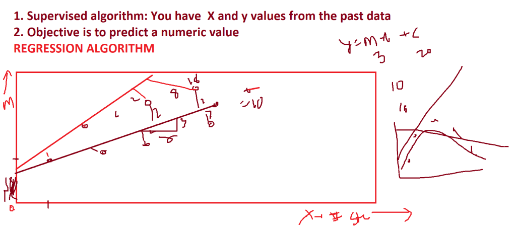
MACHINE LEARNING TUTORIAL
link =“https://raw.githubusercontent.com/swapnilsaurav/MachineLearning/master/1_Data_PreProcessing.csv”
import numpy as np
import pandas as pd
df = pd.read_csv(link)
#print(df)
X =df.iloc[:,:-1].values
y =df.iloc[:,-1].values
#print(X)
#print(y)
## 1 Handling missing values:
# a) lot of values in the rows / column – drop/delete them
# b) replace with median / mean – numeric & mode – in case of categorical
## Scikit learn package: This package does everything for machine learning
## pip install scikit-learn
# class SimpleImputer belonging to sklearn (scikit-learn) we will use to replace missing values
from sklearn.impute import SimpleImputer
imputer =SimpleImputer(missing_values=np.nan, strategy= ‘mean’)
imputer = imputer.fit(X[:,1:])
X[:,1:3] = imputer.transform(X[:,1:])
#print(X)
## 2 Handling categorical values
from sklearn.preprocessing import LabelEncoder, OneHotEncoder
from sklearn.compose import ColumnTransformer
lc = LabelEncoder()
X[:,0] = lc.fit_transform(X[:,0])
transform = ColumnTransformer([(‘one_hot_encoder’, OneHotEncoder(), [0])], remainder=‘passthrough’)
# remainder is to indicate what should columns that are not transformed be
# we are saying, let them be as it is- passthrough
X = transform.fit_transform(X)
y = lc.fit_transform(y) # y will not have ColumnTranformer
X = X[:,1:]
#print(X)
## 3 Handling Outliers
## 4 Creating Training set and Test set
from sklearn.model_selection import train_test_split
X_train, X_test, y_train, y_test = train_test_split(X,y,test_size=0.20)
## 5 Scaling
from sklearn.preprocessing import StandardScaler
sc = StandardScaler()
X_train = sc.fit_transform(X_train)
X_test = sc.fit_transform(X_test)
print(X_train, y_train, X_test,y_test)
# K-Fold Cross Validation
from sklearn.model_selection import KFold
kf = KFold(n_splits=3)
for train, test in kf.split(X):
print(“============”)
print(train, “\n“,test)
#### MODEL
import matplotlib.pyplot as plt
df = pd.read_csv(“D:/datasets/2_Marks_Data.csv”)
print(“Columns are:”,df.columns)
print(“Shape: “,df.shape)
print(“Top 5 rows are: \n“,df.head(3))
print(“Describe :\n“,df.describe())
plt.scatter(df[“Hours”], df[“Marks”])
plt.show()
X = df.iloc[:,:1].values
y = df.iloc[:,1].values
from sklearn.model_selection import train_test_split
X_train, X_test,y_train,y_test = train_test_split(X,y,test_size=0.2, random_state=1)
# running the algorithm- Simple Linear Regression
from sklearn.linear_model import LinearRegression
regressor = LinearRegression()
#train the data
regressor.fit(X_train, y_train)
#
#above model will give the line in the form mx + c
#output values
print(“Coefficient (m / slope): “, regressor.coef_)
print(“Intercept (c / constant): “, regressor.intercept_)
”’
Coefficient (m / slope): [7.47852733]
Intercept (c / constant): 20.591719221277778
Y = 7.5 * X + 20.6
”’
y_pred = regressor.predict(X_test)
result_df = pd.DataFrame({‘Actual’:y_test, ‘Predicted’:y_pred})
print(result_df)
# RMSE:
# Root (Square root)
# Mean (take the mean: sum of the square /n)
# Squared (square the difference)
# Error (difference)
from sklearn import metrics
mse = metrics.mean_squared_error(y_test, y_pred) #like variance
rmse = mse**0.5 # like std dev
print(“RMSE = “,rmse)
Regression: Output (Marks) is a continous variable
Algorithm: Simple (as it has only 1 X column) Linear (assuming that dataset is linear) Regression
X – independent variable(s)
Y – dependent variable
”’
import pandas as pd
import matplotlib.pyplot as plt
link = “https://raw.githubusercontent.com/swapnilsaurav/MachineLearning/master/2_Marks_Data.csv”
df = pd.read_csv(link)
X = df.iloc[:,:1].values
y = df.iloc[:,1].values
”’
# 1. Replace the missing values with mean value
from sklearn.impute import SimpleImputer
import numpy as np
imputer = SimpleImputer(missing_values=np.nan, strategy=’mean’)
imputer = imputer.fit(X[:,1:3])
X[:,1:3] = imputer.transform(X[:,1:3])
#print(X)
# 2. Handling categorical values
# encoding
from sklearn.preprocessing import LabelEncoder, OneHotEncoder
lc = LabelEncoder()
X[:,0] = lc.fit_transform(X[:,0])
from sklearn.compose import ColumnTransformer
transform = ColumnTransformer([(‘one_hot_encoder’, OneHotEncoder(),[0])],remainder=’passthrough’)
X=transform.fit_transform(X)
X = X[:,1:] # dropped one column
#print(X)
”’
# EDA – Exploratory Data Analysis
plt.scatter(x=df[‘Hours’],y=df[‘Marks’])
plt.show()
”’
Scatter plots – shows relationship between X and Y variables. You can have:
1. Positive correlation:
2. Negative correlation:
3. No Correlation
4. Correlation: 0 to +/- 1
5. Correlation value: 0 to +/- 0.5 : no correlation
6. Strong correlation value will be closer to +/- 1
7. Equation: straight line => y = mx + c
”’
# 3. splitting it into train and test test
from sklearn.model_selection import train_test_split
X_train, X_test, y_train, y_test = train_test_split(X,y,test_size=0.2, random_state=100)
print(X_train)
”’
# 4. Scaling / Normalization
from sklearn.preprocessing import StandardScaler
scale = StandardScaler()
X_train = scale.fit_transform(X_train[:,3:])
X_test = scale.fit_transform(X_test[:,3:])
print(X_train)
”’
## RUN THE MODEL
from sklearn.linear_model import LinearRegression
regressor = LinearRegression()
# fit – train the model
regressor.fit(X_train, y_train)
print(f”M/Coefficient/Slope = {regressor.coef_} and the Constant = {regressor.intercept_}“)
# y = 7.5709072 X + 20.1999196152844
# M/Coefficient/Slope = [7.49202113] and the Constant = 21.593606679699406
y_pred = regressor.predict(X_test)
result_df =pd.DataFrame({‘Actual’: y_test, ‘Predicted’: y_pred})
print(result_df)
# Analyze the output
from sklearn import metrics
mse = metrics.mean_squared_error(y_true=y_test, y_pred=y_pred)
print(“Root Mean Squared Error (Variance) = “,mse**0.5)
mae = metrics.mean_absolute_error(y_true=y_test, y_pred=y_pred)
print(“Mean Absolute Error = “,mae)
print(“R Square is (Variance)”,metrics.r2_score(y_test, y_pred))
## Bias is based on training data
y_pred_tr = regressor.predict(X_train)
mse = metrics.mean_squared_error(y_true=y_train, y_pred=y_pred_tr)
print(“Root Mean Squared Error (Bias) = “,mse**0.5)
print(“R Square is (Bias)”,metrics.r2_score(y_train, y_pred_tr))
## Bias v Variance
import matplotlib.pyplot as plt
link = “https://raw.githubusercontent.com/swapnilsaurav/MachineLearning/master/3_Startups.csv”
df = pd.read_csv(link)
print(df.describe())
X = df.iloc[:,:4].values
y = df.iloc[:,4].values
”’
# 1. Replace the missing values with mean value
from sklearn.impute import SimpleImputer
import numpy as np
imputer = SimpleImputer(missing_values=np.nan, strategy=’mean’)
imputer = imputer.fit(X[:,1:3])
X[:,1:3] = imputer.transform(X[:,1:3])
#print(X)
”’
# 2. Handling categorical values
# encoding
from sklearn.preprocessing import LabelEncoder, OneHotEncoder
lc = LabelEncoder()
X[:,3] = lc.fit_transform(X[:,3])
from sklearn.compose import ColumnTransformer
transform = ColumnTransformer([(‘one_hot_encoder’, OneHotEncoder(),[3])],remainder=‘passthrough’)
X=transform.fit_transform(X)
X = X[:,1:] # dropped one column
print(X)
# EDA – Exploratory Data Analysis
plt.scatter(x=df[‘Administration’],y=df[‘Profit’])
plt.show()
plt.scatter(x=df[‘R&D Spend’],y=df[‘Profit’])
plt.show()
plt.scatter(x=df[‘Marketing Spend’],y=df[‘Profit’])
plt.show()
# 3. splitting it into train and test test
from sklearn.model_selection import train_test_split
X_train, X_test, y_train, y_test = train_test_split(X,y,test_size=0.2, random_state=100)
print(X_train)
”’
# 4. Scaling / Normalization
from sklearn.preprocessing import StandardScaler
scale = StandardScaler()
X_train = scale.fit_transform(X_train[:,3:])
X_test = scale.fit_transform(X_test[:,3:])
print(X_train)
”’
## RUN THE MODEL
from sklearn.linear_model import LinearRegression
regressor = LinearRegression()
# fit – train the model
regressor.fit(X_train, y_train)
print(f”M/Coefficient/Slope = {regressor.coef_} and the Constant = {regressor.intercept_}“)
# y = -3791.2 x Florida -3090.1 x California + 0.82 R&D – 0.05 Admin + 0.022 Marketing+ 56650
y_pred = regressor.predict(X_test)
result_df =pd.DataFrame({‘Actual’: y_test, ‘Predicted’: y_pred})
print(result_df)
# Analyze the output
from sklearn import metrics
mse = metrics.mean_squared_error(y_true=y_test, y_pred=y_pred)
print(“Root Mean Squared Error (Variance) = “,mse**0.5)
mae = metrics.mean_absolute_error(y_true=y_test, y_pred=y_pred)
print(“Mean Absolute Error = “,mae)
print(“R Square is (Variance)”,metrics.r2_score(y_test, y_pred))
## Bias is based on training data
y_pred_tr = regressor.predict(X_train)
mse = metrics.mean_squared_error(y_true=y_train, y_pred=y_pred_tr)
print(“Root Mean Squared Error (Bias) = “,mse**0.5)
print(“R Square is (Bias)”,metrics.r2_score(y_train, y_pred_tr))
”’
Case 1: All the columns are taken into account:
Mean Absolute Error = 8696.887641252619
R Square is (Variance) 0.884599945166969
Root Mean Squared Error (Bias) = 7562.5657508560125
R Square is (Bias) 0.9624157828452926
”’
## Testing
import statsmodels.api as sm
import numpy as np
X = np.array(X, dtype=float)
print(“Y:\n“,y)
summ1 = sm.OLS(y,X).fit().summary()
print(“Summary of All X \n—————-\n:”,summ1)
import matplotlib.pyplot as plt
link = “https://raw.githubusercontent.com/swapnilsaurav/MachineLearning/master/3_Startups.csv”
df = pd.read_csv(link)
print(df.describe())
X = df.iloc[:,:4].values
y = df.iloc[:,4].values
”’
# 1. Replace the missing values with mean value
from sklearn.impute import SimpleImputer
import numpy as np
imputer = SimpleImputer(missing_values=np.nan, strategy=’mean’)
imputer = imputer.fit(X[:,1:3])
X[:,1:3] = imputer.transform(X[:,1:3])
#print(X)
”’
# 2. Handling categorical values
# encoding
from sklearn.preprocessing import LabelEncoder, OneHotEncoder
lc = LabelEncoder()
X[:,3] = lc.fit_transform(X[:,3])
from sklearn.compose import ColumnTransformer
transform = ColumnTransformer([(‘one_hot_encoder’, OneHotEncoder(),[3])],remainder=‘passthrough’)
X=transform.fit_transform(X)
X = X[:,1:] # dropped one column
print(X)
”’
After doing Backward elemination method we realized that all the state columns
are not significantly impacting the analysis hence removing those 2 columns too.
”’
X = X[:,2:] # after backward elemination
# EDA – Exploratory Data Analysis
plt.scatter(x=df[‘Administration’],y=df[‘Profit’])
plt.show()
plt.scatter(x=df[‘R&D Spend’],y=df[‘Profit’])
plt.show()
plt.scatter(x=df[‘Marketing Spend’],y=df[‘Profit’])
plt.show()
# 3. splitting it into train and test test
from sklearn.model_selection import train_test_split
X_train, X_test, y_train, y_test = train_test_split(X,y,test_size=0.2, random_state=100)
print(X_train)
”’
# 4. Scaling / Normalization
from sklearn.preprocessing import StandardScaler
scale = StandardScaler()
X_train = scale.fit_transform(X_train[:,3:])
X_test = scale.fit_transform(X_test[:,3:])
print(X_train)
”’
## RUN THE MODEL
from sklearn.linear_model import LinearRegression
regressor = LinearRegression()
# fit – train the model
regressor.fit(X_train, y_train)
print(f”M/Coefficient/Slope = {regressor.coef_} and the Constant = {regressor.intercept_}“)
# y = -3791.2 x Florida -3090.1 x California + 0.82 R&D – 0.05 Admin + 0.022 Marketing+ 56650
y_pred = regressor.predict(X_test)
result_df =pd.DataFrame({‘Actual’: y_test, ‘Predicted’: y_pred})
print(result_df)
# Analyze the output
from sklearn import metrics
mse = metrics.mean_squared_error(y_true=y_test, y_pred=y_pred)
print(“Root Mean Squared Error (Variance) = “,mse**0.5)
mae = metrics.mean_absolute_error(y_true=y_test, y_pred=y_pred)
print(“Mean Absolute Error = “,mae)
print(“R Square is (Variance)”,metrics.r2_score(y_test, y_pred))
## Bias is based on training data
y_pred_tr = regressor.predict(X_train)
mse = metrics.mean_squared_error(y_true=y_train, y_pred=y_pred_tr)
print(“Root Mean Squared Error (Bias) = “,mse**0.5)
print(“R Square is (Bias)”,metrics.r2_score(y_train, y_pred_tr))
”’
Case 1: All the columns are taken into account:
Mean Absolute Error = 8696.887641252619
R Square is (Variance) 0.884599945166969
Root Mean Squared Error (Bias) = 7562.5657508560125
R Square is (Bias) 0.9624157828452926
”’
## Testing
import statsmodels.api as sm
import numpy as np
X = np.array(X, dtype=float)
#X = X[:,[2,3,4]]
print(“Y:\n“,y)
summ1 = sm.OLS(y,X).fit().summary()
print(“Summary of All X \n—————-\n:”,summ1)
## Test for linearity
# 1. All features (X) should be correlated to Y
# 2. Multicollinearity: Within X there should not be any correlation,
# if its there then take any one for the analysis
import matplotlib.pyplot as plt
link = “https://raw.githubusercontent.com/swapnilsaurav/MachineLearning/master/4_Position_Salaries.csv”
df = pd.read_csv(link)
print(df.describe())
X = df.iloc[:,1:2].values
y = df.iloc[:,2].values
”’
# 1. Replace the missing values with mean value
from sklearn.impute import SimpleImputer
import numpy as np
imputer = SimpleImputer(missing_values=np.nan, strategy=’mean’)
imputer = imputer.fit(X[:,1:3])
X[:,1:3] = imputer.transform(X[:,1:3])
#print(X)
”’
”’
# 2. Handling categorical values
# encoding
from sklearn.preprocessing import LabelEncoder, OneHotEncoder
lc = LabelEncoder()
X[:,3] = lc.fit_transform(X[:,3])
from sklearn.compose import ColumnTransformer
transform = ColumnTransformer([(‘one_hot_encoder’, OneHotEncoder(),[3])],remainder=’passthrough’)
X=transform.fit_transform(X)
X = X[:,1:] # dropped one column
print(X)
”’
”’
After doing Backward elemination method we realized that all the state columns
are not significantly impacting the analysis hence removing those 2 columns too.
X = X[:,2:] # after backward elemination
”’
”’
# EDA – Exploratory Data Analysis
plt.scatter(x=df[‘Level’],y=df[‘Salary’])
plt.show()
”’
# 3. splitting it into train and test test
from sklearn.model_selection import train_test_split
X_train, X_test, y_train, y_test = train_test_split(X,y,test_size=0.3, random_state=100)
print(X_train)
from sklearn.linear_model import LinearRegression
from sklearn import metrics
”’
# 4. Scaling / Normalization
from sklearn.preprocessing import StandardScaler
scale = StandardScaler()
X_train = scale.fit_transform(X_train[:,3:])
X_test = scale.fit_transform(X_test[:,3:])
print(X_train)
”’
”’
#Since dataset is too small, lets take entire data for training
X_train, y_train = X,y
X_test, y_test = X,y
”’
”’
## RUN THE MODEL
regressor = LinearRegression()
# fit – train the model
regressor.fit(X_train, y_train)
print(f”M/Coefficient/Slope = {regressor.coef_} and the Constant = {regressor.intercept_}”)
# y =
y_pred = regressor.predict(X_test)
result_df =pd.DataFrame({‘Actual’: y_test, ‘Predicted’: y_pred})
print(result_df)
# Analyze the output
mse = metrics.mean_squared_error(y_true=y_test, y_pred=y_pred)
print(“Root Mean Squared Error (Variance) = “,mse**0.5)
mae = metrics.mean_absolute_error(y_true=y_test, y_pred=y_pred)
print(“Mean Absolute Error = “,mae)
print(“R Square is (Variance)”,metrics.r2_score(y_test, y_pred))
## Bias is based on training data
y_pred_tr = regressor.predict(X_train)
mse = metrics.mean_squared_error(y_true=y_train, y_pred=y_pred_tr)
print(“Root Mean Squared Error (Bias) = “,mse**0.5)
print(“R Square is (Bias)”,metrics.r2_score(y_train, y_pred_tr))
# Plotting the data for output
plt.scatter(x=df[‘Level’],y=df[‘Salary’])
plt.plot(X,y_pred)
plt.xlabel(“Level”)
plt.ylabel(“Salary”)
plt.show()
”’
# 3. Model – Polynomial regression analysis
# y = C + m1 * X + m2 * x square
from sklearn.preprocessing import PolynomialFeatures
from sklearn.pipeline import Pipeline
for i in range(1,10):
#prepare the parameters
parameters = [(‘polynomial’, PolynomialFeatures(degree=i)),(‘modal’,LinearRegression())]
pipe = Pipeline(parameters)
pipe.fit(X_train,y_train)
y_pred = pipe.predict(X)
## Bias is based on training data
y_pred_tr = pipe.predict(X_train)
mse = metrics.mean_squared_error(y_true=y_train, y_pred=y_pred_tr)
rmse_tr = mse ** 0.5
print(“Root Mean Squared Error (Bias) = “,rmse_tr)
print(“R Square is (Bias)”,metrics.r2_score(y_train, y_pred_tr))
## Variance is based on validation data
y_pred_tt = pipe.predict(X_test)
mse = metrics.mean_squared_error(y_true=y_test, y_pred=y_pred_tt)
rmse_tt = mse ** 0.5
print(“Root Mean Squared Error (Variance) = “, rmse_tt)
print(“R Square is (Variance)”, metrics.r2_score(y_test, y_pred_tt))
print(“Difference Between variance and bias = “,rmse_tt – rmse_tr)
# Plotting the data for output
plt.scatter(x=df[‘Level’],y=df[‘Salary’])
plt.plot(X,y_pred)
plt.title(“Polynomial Analysis degree =”+str(i))
plt.xlabel(“Level”)
plt.ylabel(“Salary”)
plt.show()
import matplotlib.pyplot as plt
#link = “https://raw.githubusercontent.com/swapnilsaurav/MachineLearning/master/4_Position_Salaries.csv”
link = “https://raw.githubusercontent.com/swapnilsaurav/MachineLearning/master/3_Startups.csv”
df = pd.read_csv(link)
print(df.describe())
X = df.iloc[:,0:4].values
y = df.iloc[:,4].values
”’
# 1. Replace the missing values with mean value
from sklearn.impute import SimpleImputer
import numpy as np
imputer = SimpleImputer(missing_values=np.nan, strategy=’mean’)
imputer = imputer.fit(X[:,1:3])
X[:,1:3] = imputer.transform(X[:,1:3])
#print(X)
”’
# 2. Handling categorical values
# encoding
from sklearn.preprocessing import LabelEncoder, OneHotEncoder
lc = LabelEncoder()
X[:,3] = lc.fit_transform(X[:,3])
from sklearn.compose import ColumnTransformer
transform = ColumnTransformer([(‘one_hot_encoder’, OneHotEncoder(),[3])],remainder=‘passthrough’)
X=transform.fit_transform(X)
X = X[:,1:] # dropped one column
print(X)
”’
After doing Backward elemination method we realized that all the state columns
are not significantly impacting the analysis hence removing those 2 columns too.
X = X[:,2:] # after backward elemination
”’
”’
# EDA – Exploratory Data Analysis
plt.scatter(x=df[‘Level’],y=df[‘Salary’])
plt.show()
”’
# 3. splitting it into train and test test
from sklearn.model_selection import train_test_split
X_train, X_test, y_train, y_test = train_test_split(X,y,test_size=0.3, random_state=100)
print(X_train)
from sklearn.linear_model import LinearRegression
from sklearn import metrics
”’
# 4. Scaling / Normalization
from sklearn.preprocessing import StandardScaler
scale = StandardScaler()
X_train = scale.fit_transform(X_train[:,3:])
X_test = scale.fit_transform(X_test[:,3:])
print(X_train)
”’
”’
#Since dataset is too small, lets take entire data for training
X_train, y_train = X,y
X_test, y_test = X,y
”’
## RUN THE MODEL – Support Vector Machine Regressor (SVR)
from sklearn.svm import SVR
#regressor = SVR(kernel=’linear’)
#regressor = SVR(kernel=’poly’,degree=2,C=10)
# Assignment – Best value for gamma: 0.01 to 1 (0.05)
regressor = SVR(kernel=“rbf”,gamma=0.1,C=10)
# fit – train the model
regressor.fit(X_train, y_train)
# y =
y_pred = regressor.predict(X_test)
result_df =pd.DataFrame({‘Actual’: y_test, ‘Predicted’: y_pred})
print(result_df)
# Analyze the output
mse = metrics.mean_squared_error(y_true=y_test, y_pred=y_pred)
print(“Root Mean Squared Error (Variance) = “,mse**0.5)
mae = metrics.mean_absolute_error(y_true=y_test, y_pred=y_pred)
print(“Mean Absolute Error = “,mae)
print(“R Square is (Variance)”,metrics.r2_score(y_test, y_pred))
## Bias is based on training data
y_pred_tr = regressor.predict(X_train)
mse = metrics.mean_squared_error(y_true=y_train, y_pred=y_pred_tr)
print(“Root Mean Squared Error (Bias) = “,mse**0.5)
print(“R Square is (Bias)”,metrics.r2_score(y_train, y_pred_tr))
# Plotting the data for output
plt.scatter(X_train[:,2],y_pred_tr)
#plt.plot(X_train[:,2],y_pred_tr)
plt.show()
import pandas as pd
link = “https://raw.githubusercontent.com/swapnilsaurav/MachineLearning/master/3_Startups.csv”
link = “D:\\datasets\\3_Startups.csv”
df = pd.read_csv(link)
print(df)
#X = df.iloc[:,:4].values
X = df.iloc[:,:1].values
y = df.iloc[:,:-1].values
from sklearn.model_selection import train_test_split
X_train, X_test,y_train,y_test = train_test_split(X,y,test_size=0.25,random_state=100)
from sklearn.tree import DecisionTreeRegressor
regressor = DecisionTreeRegressor()
regressor.fit(X_train,y_train)
y_pred = regressor.predict(X_test)
# Baging, Boosting, Ensemble
from sklearn.ensemble import RandomForestRegressor
regressor = RandomForestRegressor(n_estimators=10)
regressor.fit(X_train,y_train)
y_pred = regressor.predict(X_test)
## Assignment these algorithms and check the RMSE and R square values for both of these algorithms
import pandas as pd
link=“https://raw.githubusercontent.com/swapnilsaurav/Dataset/master/student_scores_multi.csv”
df = pd.read_csv(link)
print(df)
X = df.iloc[:,0:3].values
y = df.iloc[:,3].values
from sklearn.model_selection import train_test_split
X_train, X_test, y_train, y_test = train_test_split(X,y,test_size=0.85, random_state=100)
from sklearn.linear_model import LinearRegression, Ridge, Lasso, ElasticNet
lr_ridge = Ridge(alpha=0.8)
lr_ridge.fit(X_train,y_train)
y_ridge_pred = lr_ridge.predict(X_test)
from sklearn.metrics import r2_score
r2_ridge_test = r2_score(y_test, y_ridge_pred)
y_ridge_pred_tr = lr_ridge.predict(X_train)
r2_ridge_train = r2_score(y_train, y_ridge_pred_tr)
print(f”Ridge Regression: Train R2 = {r2_ridge_train} and Test R2={r2_ridge_test}“)
”’
classifier: algorithm that we develop
model: training and predicting the outcome
features: the input data (columns)
target: class that we need to predict
classification: binary (2 class outcome) or multiclass (more than 2 classes)
Steps to run the model:
1. get the data
2. preprocess the data
3. eda
4. train the model
5. predict the model
6. evaluate the model
”’
#1. Logistic regression
link = “https://raw.githubusercontent.com/swapnilsaurav/MachineLearning/master/5_Ads_Success.csv”
import pandas as pd
df = pd.read_csv(link)
X = df.iloc[:,1:4].values
y = df.iloc[:,4].values
from sklearn.preprocessing import LabelEncoder
lc = LabelEncoder()
X[:,0] = lc.fit_transform(X[:,0] )
from sklearn.model_selection import train_test_split
X_train, X_test, y_train, y_test = train_test_split(X,y,test_size=0.25, random_state=100)
# Scaling as Age and Salary are in different range of values
from sklearn.preprocessing import StandardScaler
sc = StandardScaler()
X_train = sc.fit_transform(X_train)
X_test = sc.fit_transform(X_test)
## Build the model
from sklearn.linear_model import LogisticRegression
classifier = LogisticRegression()
classifier.fit(X_train,y_train)
y_pred = classifier.predict(X_test)
# visualize the outcome
X_train = X_train[:,1:]
X_test = X_test[:,1:]
classifier.fit(X_train,y_train)
y_pred = classifier.predict(X_test)
from matplotlib.colors import ListedColormap
import matplotlib.pyplot as plt
import numpy as np
x_set, y_set = X_train, y_train
X1,X2 = np.meshgrid(np.arange(start = x_set[:,0].min()-1, stop=x_set[:,0].max()+1, step=0.01),
np.arange(start = x_set[:,1].min()-1, stop=x_set[:,1].max()+1, step=0.01))
plt.contourf(X1,X2,classifier.predict(np.array([X1.ravel(),X2.ravel()]).T).reshape(X1.shape),
cmap=ListedColormap((‘red’,‘green’)))
plt.show()
”’
classifier: algorithm that we develop
model: training and predicting the outcome
features: the input data (columns)
target: class that we need to predict
classification: binary (2 class outcome) or multiclass (more than 2 classes)
Steps to run the model:
1. get the data
2. preprocess the data
3. eda
4. train the model
5. predict the model
6. evaluate the model
”’
#1. Logistic regression
link = “https://raw.githubusercontent.com/swapnilsaurav/MachineLearning/master/5_Ads_Success.csv”
link = “D:\\datasets\\5_Ads_Success.csv”
import pandas as pd
df = pd.read_csv(link)
X = df.iloc[:,1:4].values
y = df.iloc[:,4].values
from sklearn.preprocessing import LabelEncoder
lc = LabelEncoder()
X[:,0] = lc.fit_transform(X[:,0] )
from sklearn.model_selection import train_test_split
X_train, X_test, y_train, y_test = train_test_split(X,y,test_size=0.25, random_state=100)
# Scaling as Age and Salary are in different range of values
from sklearn.preprocessing import StandardScaler
sc = StandardScaler()
X_train = sc.fit_transform(X_train)
X_test = sc.fit_transform(X_test)
## Build the model
”’
## LOGISTIC REGRESSION
from sklearn.linear_model import LogisticRegression
classifier = LogisticRegression()
classifier.fit(X_train,y_train)
y_pred = classifier.predict(X_test)
”’
from sklearn.svm import SVC
”’
## Support Vector Machine – Classifier
classifier = SVC(kernel=’linear’)
classifier = SVC(kernel=’rbf’,gamma=100, C=100)
”’
from sklearn.neighbors import KNeighborsClassifier
## Refer types of distances:
# https://designrr.page/?id=200944&token=2785938662&type=FP&h=7229
classifier = KNeighborsClassifier(n_neighbors=9, metric=‘minkowski’)
classifier.fit(X_train,y_train)
y_pred = classifier.predict(X_test)
# visualize the outcome
X_train = X_train[:,1:]
X_test = X_test[:,1:]
classifier.fit(X_train,y_train)
y_pred = classifier.predict(X_test)
from matplotlib.colors import ListedColormap
import matplotlib.pyplot as plt
import numpy as np
x_set, y_set = X_train, y_train
X1,X2 = np.meshgrid(np.arange(start = x_set[:,0].min()-1, stop=x_set[:,0].max()+1, step=0.01),
np.arange(start = x_set[:,1].min()-1, stop=x_set[:,1].max()+1, step=0.01))
plt.contourf(X1,X2,classifier.predict(np.array([X1.ravel(),X2.ravel()]).T).reshape(X1.shape),
cmap=ListedColormap((‘red’,‘green’)))
#Now we will plot training data
for i, j in enumerate(np.unique(y_set)):
plt.scatter(x_set[y_set==j,0],
x_set[y_set==j,1], color=ListedColormap((“red”,“green”))(i),
label=j)
plt.show()
## Model Evaluation using Confusion Matrix
from sklearn.metrics import classification_report, confusion_matrix, accuracy_score
cm = confusion_matrix(y_test, y_pred)
print(“Confusion Matrix: \n“,cm)
cr = classification_report(y_test, y_pred)
accs = accuracy_score(y_test, y_pred)
print(“classification_report: \n“,cr)
print(“accuracy_score: “,accs)
link = “https://raw.githubusercontent.com/swapnilsaurav/MachineLearning/master/5_Ads_Success.csv”
link = “D:\\datasets\\5_Ads_Success.csv”
import pandas as pd
df = pd.read_csv(link)
X = df.iloc[:,1:4].values
y = df.iloc[:,4].values
from sklearn.preprocessing import LabelEncoder
lc = LabelEncoder()
X[:,0] = lc.fit_transform(X[:,0] )
from sklearn.model_selection import train_test_split
X_train, X_test, y_train, y_test = train_test_split(X,y,test_size=0.25, random_state=100)
# Scaling as Age and Salary are in different range of values
from sklearn.preprocessing import StandardScaler
sc = StandardScaler()
X_train = sc.fit_transform(X_train)
X_test = sc.fit_transform(X_test)
## Build the model
”’
from sklearn.tree import DecisionTreeClassifier
classifier = DecisionTreeClassifier(criterion=”gini”)
”’
from sklearn.ensemble import RandomForestClassifier
classifier = RandomForestClassifier(n_estimators=39, criterion=“gini”)
classifier.fit(X_train,y_train)
y_pred = classifier.predict(X_test)
# visualize the outcome
X_train = X_train[:,1:]
X_test = X_test[:,1:]
classifier.fit(X_train,y_train)
y_pred = classifier.predict(X_test)
from matplotlib.colors import ListedColormap
import matplotlib.pyplot as plt
import numpy as np
x_set, y_set = X_train, y_train
X1,X2 = np.meshgrid(np.arange(start = x_set[:,0].min()-1, stop=x_set[:,0].max()+1, step=0.01),
np.arange(start = x_set[:,1].min()-1, stop=x_set[:,1].max()+1, step=0.01))
plt.contourf(X1,X2,classifier.predict(np.array([X1.ravel(),X2.ravel()]).T).reshape(X1.shape),
cmap=ListedColormap((‘red’,‘green’)))
#Now we will plot training data
for i, j in enumerate(np.unique(y_set)):
plt.scatter(x_set[y_set==j,0],
x_set[y_set==j,1], color=ListedColormap((“red”,“green”))(i),
label=j)
plt.show()
## Model Evaluation using Confusion Matrix
from sklearn.metrics import classification_report, confusion_matrix, accuracy_score
cm = confusion_matrix(y_test, y_pred)
print(“Confusion Matrix: \n“,cm)
cr = classification_report(y_test, y_pred)
accs = accuracy_score(y_test, y_pred)
print(“classification_report: \n“,cr)
print(“accuracy_score: “,accs)
”’
# Show decision tree created
output = sklearn.tree.export_text(classifier)
print(output)
# visualize the tree
fig = plt.figure(figsize=(40,60))
tree_plot = sklearn.tree.plot_tree(classifier)
plt.show()
”’
”’
In Ensemble Algorithms – we run multiple algorithms to improve the performance
of a given business objective:
1. Boosting: When you run same algorithm – Input varies based on weights
2. Bagging: When you run same algorithm – average of all
3. Stacking: Over different algorithms – average of all
”’
link = “https://raw.githubusercontent.com/swapnilsaurav/MachineLearning/master/5_Ads_Success.csv”
link = “D:\\datasets\\5_Ads_Success.csv”
import pandas as pd
df = pd.read_csv(link)
X = df.iloc[:,1:4].values
y = df.iloc[:,4].values
from sklearn.preprocessing import LabelEncoder
lc = LabelEncoder()
X[:,0] = lc.fit_transform(X[:,0] )
from sklearn.model_selection import train_test_split
X_train, X_test, y_train, y_test = train_test_split(X,y,test_size=0.25, random_state=100)
# Scaling as Age and Salary are in different range of values
from sklearn.preprocessing import StandardScaler
sc = StandardScaler()
X_train = sc.fit_transform(X_train)
X_test = sc.fit_transform(X_test)
## Build the model
”’
from sklearn.tree import DecisionTreeClassifier
classifier = DecisionTreeClassifier(criterion=”gini”)
from sklearn.ensemble import RandomForestClassifier
classifier = RandomForestClassifier(n_estimators=39, criterion=”gini”)
”’
from sklearn.ensemble import AdaBoostClassifier
classifier = AdaBoostClassifier(n_estimators=7)
classifier.fit(X_train,y_train)
y_pred = classifier.predict(X_test)
# visualize the outcome
X_train = X_train[:,1:]
X_test = X_test[:,1:]
classifier.fit(X_train,y_train)
y_pred = classifier.predict(X_test)
from matplotlib.colors import ListedColormap
import matplotlib.pyplot as plt
import numpy as np
x_set, y_set = X_train, y_train
X1,X2 = np.meshgrid(np.arange(start = x_set[:,0].min()-1, stop=x_set[:,0].max()+1, step=0.01),
np.arange(start = x_set[:,1].min()-1, stop=x_set[:,1].max()+1, step=0.01))
plt.contourf(X1,X2,classifier.predict(np.array([X1.ravel(),X2.ravel()]).T).reshape(X1.shape),
cmap=ListedColormap((‘red’,‘green’)))
#Now we will plot training data
for i, j in enumerate(np.unique(y_set)):
plt.scatter(x_set[y_set==j,0],
x_set[y_set==j,1], color=ListedColormap((“red”,“green”))(i),
label=j)
plt.show()
## Model Evaluation using Confusion Matrix
from sklearn.metrics import classification_report, confusion_matrix, accuracy_score
cm = confusion_matrix(y_test, y_pred)
print(“Confusion Matrix: \n“,cm)
cr = classification_report(y_test, y_pred)
accs = accuracy_score(y_test, y_pred)
print(“classification_report: \n“,cr)
print(“accuracy_score: “,accs)
”’
# Show decision tree created
output = sklearn.tree.export_text(classifier)
print(output)
# visualize the tree
fig = plt.figure(figsize=(40,60))
tree_plot = sklearn.tree.plot_tree(classifier)
plt.show()
”’
”’
In Ensemble Algorithms – we run multiple algorithms to improve the performance
of a given business objective:
1. Boosting: When you run same algorithm – Input varies based on weights
2. Bagging: When you run same algorithm – average of all
3. Stacking: Over different algorithms – average of all
”’
from sklearn.datasets import make_blobs
import matplotlib.pyplot as plt
X,y = make_blobs(n_samples=300, n_features=3, centers=4)
plt.scatter(X[:,0], X[:,1])
plt.show()
from sklearn.cluster import KMeans
km = KMeans(n_clusters=5, init=“random”,max_iter=100)
y_cluster =km.fit_predict(X)
plt.scatter(X[y_cluster==0,0],X[y_cluster==0,1],c=“blue”,label=“Cluster A”)
plt.scatter(X[y_cluster==1,0],X[y_cluster==1,1],c=“red”,label=“Cluster B”)
plt.scatter(X[y_cluster==2,0],X[y_cluster==2,1],c=“green”,label=“Cluster C”)
plt.scatter(X[y_cluster==3,0],X[y_cluster==3,1],c=“black”,label=“Cluster D”)
plt.scatter(X[y_cluster==4,0],X[y_cluster==4,1],c=“orange”,label=“Cluster E”)
plt.show()
distortion = []
max_centers = 30
for i in range(1,max_centers):
km = KMeans(n_clusters=i, init=“random”, max_iter=100)
y_cluster = km.fit(X)
distortion.append(km.inertia_)
print(“Distortion:\n“,distortion)
plt.plot(range(1,max_centers),distortion,marker=“o”)
plt.show()
import matplotlib.pyplot as plt
link = “D:\\Datasets\\USArrests.csv”
df = pd.read_csv(link)
#print(df)
X = df.iloc[:,1:]
from sklearn.preprocessing import normalize
data = normalize(X)
data = pd.DataFrame(data)
print(data)
## plotting dendogram
import scipy.cluster.hierarchy as sch
dendo = sch.dendrogram(sch.linkage(data, method=‘ward’))
plt.axhline(y=0.7,color=“red”)
plt.show()
import pandas as pd
df = pd.read_csv(link)
print(df)
from apyori import apriori
transactions = []
for i in range(len(df)):
if i%100==0:
print(“I = “,i)
transactions.append([str(df.values[i,j]) for j in range(20)])
## remove nan from the list
print(“Transactions:\n“,transactions)
association_algo = apriori(transactions, min_confidence=0.2, min_support=0.02, min_lift=2)
print(“Association = “,list(association_algo))
Time Series Forecasting – ARIMA method
1. Read and visualize the data
2. Stationary series
3. Optimal parameters
4. Build the model
5. Prediction
”’
import pandas as pd
#Step 1: read the data
link = “D:\\datasets\\gitdataset\\AirPassengers.csv”
air_passengers = pd.read_csv(link)
”’
#Step 2: visualize the data
import plotly.express as pe
fig = pe.line(air_passengers,x=”Month”,y=”#Passengers”)
fig.show()
”’
# Cleaning the data
from datetime import datetime
air_passengers[‘Month’] = pd.to_datetime(air_passengers[‘Month’])
air_passengers.set_index(‘Month’,inplace=True)
#converting to time series data
import numpy as np
ts_log = np.log(air_passengers[‘#Passengers’])
#creating rolling period – 12 months
import matplotlib.pyplot as plt
”’
moving_avg = ts_log.rolling(12).mean
plt.plot(ts_log)
plt.plot(moving_avg)
plt.show()
”’
#Step 3: Decomposition into: trend, seasonality, error ( or residual or noise)
”’
Additive decomposition: linear combination of above 3 factors:
Y(t) =T(t) + S(t) + E(t)
Multiplicative decomposition: product of 3 factors:
Y(t) =T(t) * S(t) * E(t)
”’
from statsmodels.tsa.seasonal import seasonal_decompose
decomposed = seasonal_decompose(ts_log,model=“multiplicative”)
decomposed.plot()
plt.show()
# Step 4: Stationary test
”’
To make Time series analysis, the TS should be stationary.
A time series is said to be stationary if its statistical properties
(mean, variance, autocorrelation) doesnt change by a large value
over a period of time.
Types of tests:
1. Augmented Dickey Fuller test (ADH Test)
2. Kwiatkowski Phillips Schnidt Shin (KPSS) test
3. Phillips Perron (PP) Test
Null Hypothesis: The time series is not stationary
Alternate Hypothesis: Time series is stationary
If p >0.05 we reject Null Hypothesis
”’
from statsmodels.tsa.stattools import adfuller
result = adfuller(air_passengers[‘#Passengers’])
print(“ADF Stats: \n“,result[0])
print(“p value = “,result[1])
”’
To reject Null hypothesis, result[0] less than 5% critical region value
and p > 0.05
”’
# Run the model
”’
ARIMA model: Auto-Regressive Integrative Moving Average
AR: p predicts the current value
I: d integrative by removing trend and seasonality component from previous period
MA: q represents Moving Average
AIC- Akaike’s Information Criterion (AIC) – helps to find optimal p,d,q values
BIC – Bayesian Information Criterion (BIC) – alternative to AIC
”’
from statsmodels.graphics.tsaplots import plot_acf, plot_pacf
plot_acf(air_passengers[‘#Passengers’].diff().dropna())
plot_pacf(air_passengers[‘#Passengers’].diff().dropna())
plt.show()
”’
How to read above graph:
To find q (MA), we look at the Autocorrelation graph and see where there is a drastic change:
here, its at 1, so q = 1 (or 2 as at 2, it goes to -ve)
To find p (AR) – sharp drop in Partial Autocorrelation graph:
here, its at 1, so p = 1 (or 2 as at 2, it goes to -ve)
for d (I) – we need to try with multiple values
intially we will take as 1
”’
from statsmodels.tsa.arima.model import ARIMA
model = ARIMA(air_passengers[‘#Passengers’], order=(1,1,1))
result = model.fit()
plt.plot(air_passengers[‘#Passengers’])
plt.plot(result.fittedvalues)
plt.show()
print(“ARIMA Model Summary”)
print(result.summary())
model = ARIMA(air_passengers[‘#Passengers’], order=(4,1,4))
result = model.fit()
plt.plot(air_passengers[‘#Passengers’])
plt.plot(result.fittedvalues)
plt.show()
print(“ARIMA Model Summary”)
print(result.summary())
# Prediction using ARIMA model
air_passengers[‘Forecasted’] = result.predict(start=120,end=246)
air_passengers[[‘#Passengers’,‘Forecasted’]].plot()
plt.show()
# predict using SARIMAX Model
import statsmodels.api as sm
model = sm.tsa.statespace.SARIMAX(air_passengers[‘#Passengers’],order=(7,1,1), seasonal_order=(1,1,1,12))
result = model.fit()
air_passengers[‘Forecast_SARIMAX’] = result.predict(start=120,end=246)
air_passengers[[‘#Passengers’,‘Forecast_SARIMAX’]].plot()
plt.show()
NLP – Natural Language Processing – analysing review comment to understand
reasons for positive and negative ratings.
concepts like: unigram, bigram, trigram
Steps we generally perform with NLP data:
1. Convert into lowercase
2. decompose (non unicode to unicode)
3. removing accent: encode the content to ascii values
4. tokenization: will break sentence to words
5. Stop words: not important words for analysis
6. Lemmetization (done only on English words): convert the words into dictionary words
7. N-grams: set of one word (unigram), two words (bigram), three words (trigrams)
8. Plot the graph based on the number of occurrences and Evaluate
”’
”’
cardboard mousepad. Going worth price! Not bad
”’
link=“https://raw.githubusercontent.com/swapnilsaurav/OnlineRetail/master/order_reviews.csv”
import pandas as pd
import unicodedata
import nltk
import matplotlib.pyplot as plt
df = pd.read_csv(link)
print(list(df.columns))
”’
[‘review_id’, ‘order_id’, ‘review_score’, ‘review_comment_title’,
‘review_comment_message’, ‘review_creation_date’, ‘review_answer_timestamp’]
”’
df[‘review_creation_date’] = pd.to_datetime(df[‘review_creation_date’])
df[‘review_answer_timestamp’] = pd.to_datetime(df[‘review_answer_timestamp’])
# data preprocessing – making data ready for analysis
reviews_df = df[df[‘review_comment_message’].notnull()].copy()
#print(reviews_df)
”’
Write a function to perform basic preprocessing steps
”’
def basic_preprocessing(text):
txt_pp = text.lower()
print(txt_pp)
#remove accent
# applying basic preprocessing:
reviews_df[‘review_comment_message’] = \
reviews_df[‘review_comment_message’].apply(basic_preprocessing)
NLP – Natural Language Processing – analysing review comment to understand
reasons for positive and negative ratings.
concepts like: unigram, bigram, trigram
Steps we generally perform with NLP data:
1. Convert into lowercase
2. decompose (non unicode to unicode)
3. removing accent: encode the content to ascii values
4. tokenization: will break sentence to words
5. Stop words: not important words for analysis
6. Lemmetization (done only on English words): convert the words into dictionary words
7. N-grams: set of one word (unigram), two words (bigram), three words (trigrams)
8. Plot the graph based on the number of occurrences and Evaluate
”’
”’
cardboard mousepad. Going worth price! Not bad
”’
link=“D:/datasets/OnlineRetail/order_reviews.csv”
import pandas as pd
import unicodedata
import nltk
import matplotlib.pyplot as plt
df = pd.read_csv(link)
print(list(df.columns))
”’
[‘review_id’, ‘order_id’, ‘review_score’, ‘review_comment_title’,
‘review_comment_message’, ‘review_creation_date’, ‘review_answer_timestamp’]
”’
#df[‘review_creation_date’] = pd.to_datetime(df[‘review_creation_date’])
#df[‘review_answer_timestamp’] = pd.to_datetime(df[‘review_answer_timestamp’])
# data preprocessing – making data ready for analysis
reviews_df = df[df[‘review_comment_message’].notnull()].copy()
#print(reviews_df)
# remove accents
def remove_accent(text):
return unicodedata.normalize(‘NFKD’,text).encode(‘ascii’,errors=‘ignore’).decode(‘utf-8’)
#STOP WORDS LIST:
STOP_WORDS = set(remove_accent(w) for w in nltk.corpus.stopwords.words(‘portuguese’))
”’
Write a function to perform basic preprocessing steps
”’
def basic_preprocessing(text):
#converting to lower case
txt_pp = text.lower()
#print(txt_pp)
#remove the accent
#txt_pp = unicodedata.normalize(‘NFKD’,txt_pp).encode(‘ascii’,errors=’ignore’).decode(‘utf-8’)
txt_pp =remove_accent(txt_pp)
#print(txt_pp)
#tokenize
txt_token = nltk.tokenize.word_tokenize(txt_pp)
#print(txt_token)
# removing stop words
txt_token = (w for w in txt_token if w not in STOP_WORDS and w.isalpha())
return txt_token
# applying basic preprocessing:
reviews_df[‘review_comment_words’] = \
reviews_df[‘review_comment_message’].apply(basic_preprocessing)
#get positive reviews – all 5 ratings in review_score
reviews_5 = reviews_df[reviews_df[‘review_score’]==5]
#get negative reviews – all 1 ratings
reviews_1 = reviews_df[reviews_df[‘review_score’]==1]
## write a function to creaet unigram, bigram, trigram
def create_ngrams(words):
unigram,bigrams,trigram = [],[],[]
for comment in words:
unigram.extend(comment)
bigrams.extend(”.join(bigram) for bigram in nltk.bigrams(comment))
trigram.extend(‘ ‘.join(trigram) for trigram in nltk.trigrams(comment))
return unigram,bigrams,trigram
#create ngrams for rating 5 and rating 1
uni_5, bi_5, tri_5 = create_ngrams(reviews_5[‘review_comment_words’])
print(uni_5)
print(‘””””””””””””””””””‘)
print(bi_5)
print(” =========================================”)
print(tri_5)
uni_1, bi_1, tri_1 = create_ngrams(reviews_1[‘review_comment_words’])
#print(uni_5)
# distribution plot
def plot_dist(words, color):
nltk.FreqDist(words).plot()