Maintaining a GitHub data science portfolio is very essential for data science professionals and students in their career. This will essentially showcase their skills and projects.
Steps to add an existing Machine Learning Project in GitHub
Step 1: Install GIT on your system
We will use the git command-line interface which can be downloaded from:
Step 3: Now we create a repository for our project. It’s always a good practice to initialize the project with a README file.
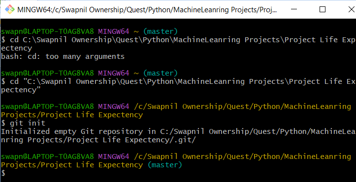
Step 4: Go to the Git folder located in Program Files\Git and open the git-bash terminal.
Step 5: Now navigate to the Machine Learning project folder using the following command.
cd PATH_TO_ML_PROJECT
Step 6: Type the following git initialization command to initialize the folder as a local git repository.
git init
We should get a message “Initialized empty Git repository in your path” and .git folder will be created which is hidden by default.
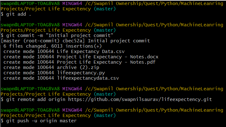
Step 7: Add files to the staging area for committing using this command which adds all the files and folders in your ML project folder.
git add .
Note: git add filename.extension can also be used to add individual files.
Step 8: We will now commit the file from the staging area and add a message to our commit. It is always a good practice to having meaningful commit messages which will help us understand the commits during future visits and revision. Type the following command for your first commit.
git commit -m "Initial project commit"
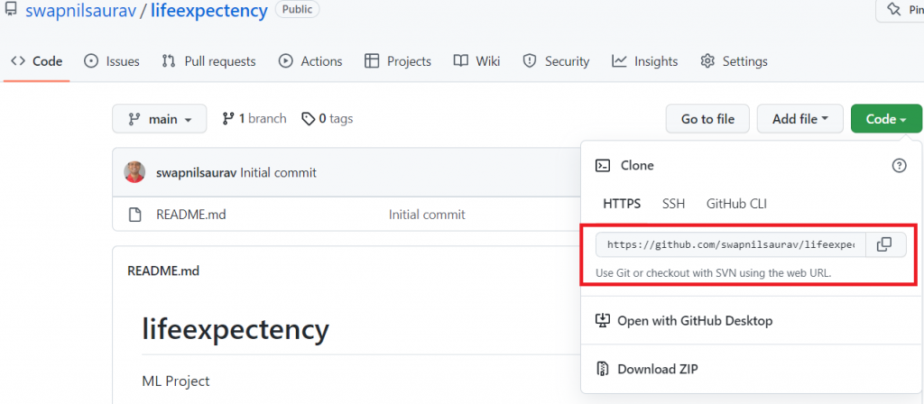
Step 9: This only adds our files to the local branch of our system and we have to link with our remote repository in GitHub. To link them go to the GitHub repository we have created earlier and copy the remote link under “..or push an existing repository from the command line”.
First, get the url of the github project:
Now, In the git-bash window, paste the command below followed by your remote repository’s URL.
git remote add origin YOUR_REMOTE_REPOSITORY_URL
Step 10: Finally, we have to push the local repository to the remote repository in GitHub
git push -u origin master
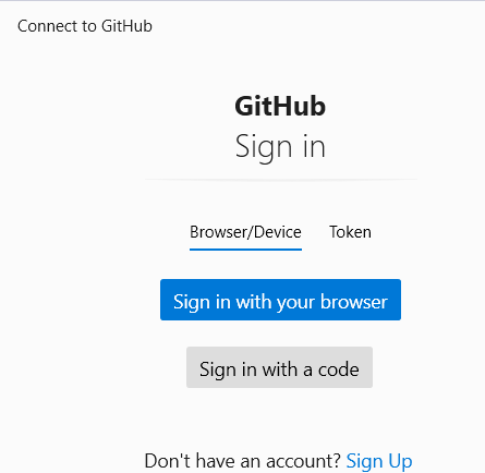
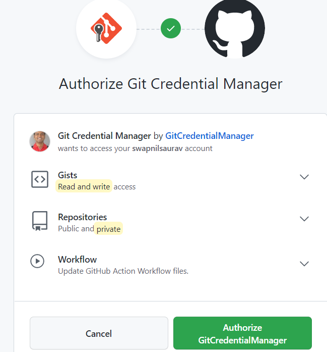
Sign into your github account
Authorize GitCredentialManager
After this, the Machine Learning project will be added to your GitHub with the files.
We have successfully added an existing Machine Learning Project to GitHub. Now is the time to create your GitHub portfolio by adding more projects to it.
Join the love revolution in re-Evolution Coffee houses!
Press release:
The next revolutionary step in the evolution of coffee house culture is the way you get your coffee. Re-Evolution Coffee shops chain MD Dirk Dash explains: “If you’d rather not queue up for your coffee at the counter, at re-Evolution Coffee Houses up and down the UK you will be able to just sit yourself down, relax and our service staff will be at your side ready to take your order, sending it instantly to the re-Evolution Coffee Wizards who will work their magic and notify the staff to deliver it to you – effortlessly… our service staff will be using the latest and best wireless technology to provide the ultimate coffee house customer experience, so relax and join the love revolution – but only in re-Evolution Coffee Houses!”
Email
From:
Dirk Dash (MD re-Evolution Coffee Houses)
to:
Adele Ash (Sales & Service Director)
Ben Bash (IT Director)
Carla Cash (Finance Director)
Subject: at seat service development & launch
Guys,
Check out the attached press release – as you know we are planning to launch in 3 months so it’s time to crack on and get this delivered.
This is a big venture for us, but it differentiates us from the competition and, if we get it right, we can get the lead in the market place…so there is a need for speed but given the likely costs and risks – money and reputation – we need to get it right first time or our shareholders will unimpressed.
As the management board, we just can’t afford another experience like the Streamline implementation.
Adele: you will need new staff and the existing ones are going to have to learn new ways of working with new technology – but this is all about customer service so make sure you let Ben know what the technology needs to do to enable your staff to deliver that service.
Ben: the wireless order taking and fulfilment capability is the backbone of this. The ‘at seat’ staff taking orders at seat can do the best job in the world but the Wizards must get the right orders in the right sequence at the right time or the ‘at seat’ staff can’t deliver excellent service.
Ben, Adele: you need to tell Carla what the indicative costs and timescales are going to be.
Carla: this initiative is key to company growth plans but not at any price, let me know as soon as you have some figures of costs and returns to show me.
This is a high risk, high reward opportunity – do it right!
Regards,
Dirk
Email
From:
Ben Bash (IT Director)
To:
Dirk Dash (MD re-Evolution Coffee Houses)
Adele Ash (Sales & Service Director)
Carla Cash (Finance Director)
Subject: Re: at seat service development & launch
Hi,
If we are going to avoid another Streamline fiasco, I suggest we start by defining exactly what it is that we’re changing in terms of systems and people. I have some business analysts already started on this to define the requirements, please make sure you make time for them.
Once we know what we’re doing here we can specify the technicalities of the wireless solution. At that point I can give some sensible cost estimates.
There is a lot we need to agree. For example one question I already have (and that makes a big difference to costs) is do we expect seated customers to be able to pay for their orders as they place them like those queuing at the counter do? We can do that but it means linking up to Streamline services via the order taking handheld and that will involve costs.
There are a shed load more questions like that which need to be answered before we can give Carla indicative costs.
Regards,
Ben
Email
From:
Adele Ash (Sales & Service Director)
To:
Dirk Dash (MD re-Evolution Coffee Houses)
Ben Bash (IT Director)
Carla Cash (Finance Director)
Subject: Re: at seat service development & launch
Hi,
Glad to hear about the business analysts, Ben. I don’t want to go through another change like StreamlineJ! We will make available as much time as needed.
Overall I can tell you how it will work right now: A customer comes in to a shop and takes a seat. The waiting staff will give them time to select what they want and then approach to take their order, coming back if necessary. While they are taking the customer order they will recommend the promotions we are running as the opportunity allows. Once they have got the order it needs to be sent to the Wizards who will make up the orders in the sequence they receive them interspersed with counter orders. Ben – can the counter orders and table orders be put on one list so the Wizards don’t have to sort through two lists? When the order is ready the Wizards need to be able to tell the waiting staff who will pick the order up from the counter and deliver.
One thing to factor in here is recruitment of new staff, and training new and existing staff. Suggest we go for a train the trainer approach and I will draw up plans accordingly.
Payment – my belief is payments will have to be made at the counter (if agreed we could look at setting up a separate payment queue for this). I think taking payment as customers place the order will take up too much time and over complicate things.
Maybe make that a next stage thing?
Regards,
Adele
Email
From:
Carla Cash (Finance Director)
To:
Dirk Dash (MD re-Evolution Coffee Houses)
Adele Ash (Sales & Service Director)
Ben Bash (IT Director)
Subject: Re: at seat service development & launch
Hi,
Ben, Adele, give me costs and benefits whenever you can, caveat them however you like. We can start building a benefits case as soon as we have some figures and then refine them as we go.
By the way, we have an opportunity here to get some good management information – things like better shop performance figures and new information like average order fulfilment time, promotions uptakes and so on. It might even be worth tracking individual staff performance…is this going to be possible? The benefits would be much better reactive management of local issues and much better future planning by shop and for the whole chain…
Regards,
Carla
Email
From:
Dirk Dash (MD re-Evolution Coffee Houses)
To:
Adele Ash (Sales & Service Director)
Ben Bash (IT Director)
Carla Cash (Finance Director)
Subject: Re: at seat service development & launch
Guys,
Great start!
I would like a presentation of how we see all this working in 3 weeks. Just show me the overall solution not the detail.
To answer some of the questions that have already come up:
Payment taking at seat is out – we’ll make it next stage as Adele suggests
Management information is in: you’re right Carla it’s a great opportunity!
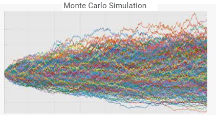
Monte Carlo simulation is a computerized mathematical technique to generate random sample data based on some known distribution for numerical experiments. This method is applied to risk quantitative analysis and decision making problems. This method is used by the professionals of various profiles such as finance, project management, energy, manufacturing, engineering, research & development, insurance, oil & gas, transportation, etc.
This method was first used by scientists working on the atom bomb in 1940. This method can be used in those situations where we need to make an estimate and uncertain decisions such as weather forecast predictions.
The Monte Carlo Simulation Formula
We would like to accurately estimate the probabilities of uncertain events. For example, what is the probability that a new product’s cash flows will have a positive net present value (NPV)? What is the risk factor of our investment portfolio? Monte Carlo simulation enables us to model situations that present uncertainty and then play them out on a computer thousands of times.
Many companies use Monte Carlo simulation as an important part of their decision-making process. Here are some examples.
General Motors, Proctor and Gamble, Pfizer, Bristol-Myers Squibb, and Eli Lilly use simulation to estimate both the average return and the risk factor of new products. At GM, this information is used by the CEO to determine which products come to market.
GM uses simulation for activities such as forecasting net income for the corporation, predicting structural and purchasing costs, and determining its susceptibility to different kinds of risk (such as interest rate changes and exchange rate fluctuations).
Lilly uses simulation to determine the optimal plant capacity for each drug.
Proctor and Gamble uses simulation to model and optimally hedge foreign exchange risk.
Sears uses simulation to determine how many units of each product line should be ordered from suppliers—for example, the number of pairs of Dockers trousers that should be ordered this year.
Oil and drug companies use simulation to value “real options,” such as the value of an option to expand, contract, or postpone a project.
Financial planners use Monte Carlo simulation to determine optimal investment strategies for their clients’ retirement.
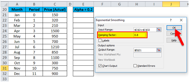
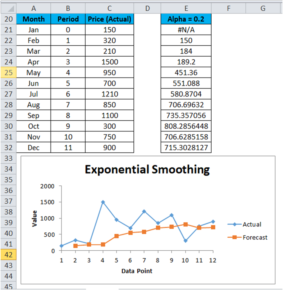
Let’s consider α=0.2 for the above-given data values so enter the value 0.8 in the Damping Factor box and again repeat the Exponential
The result is shown below:
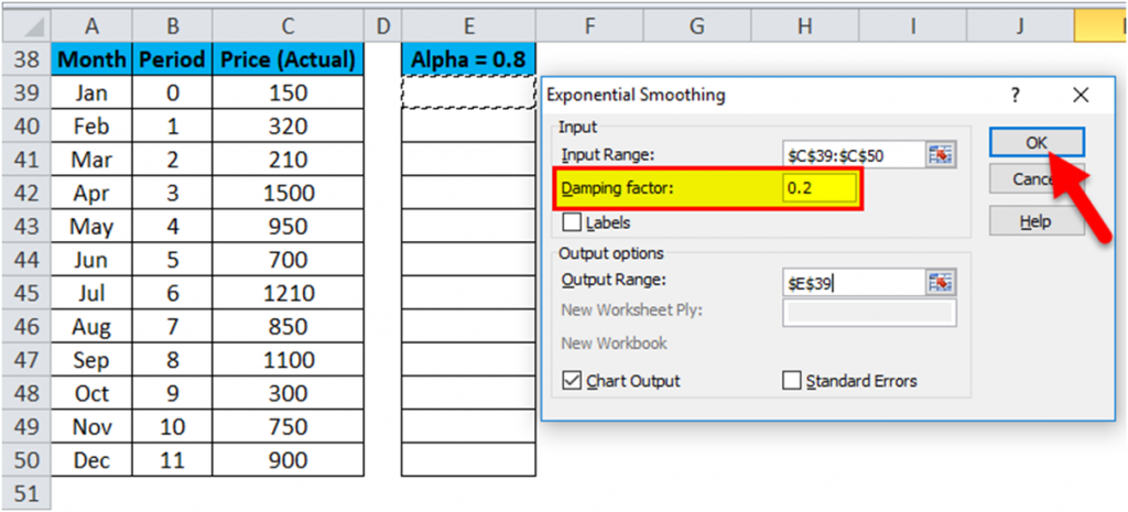
Exponential Smoothing Forecasting – Example #2
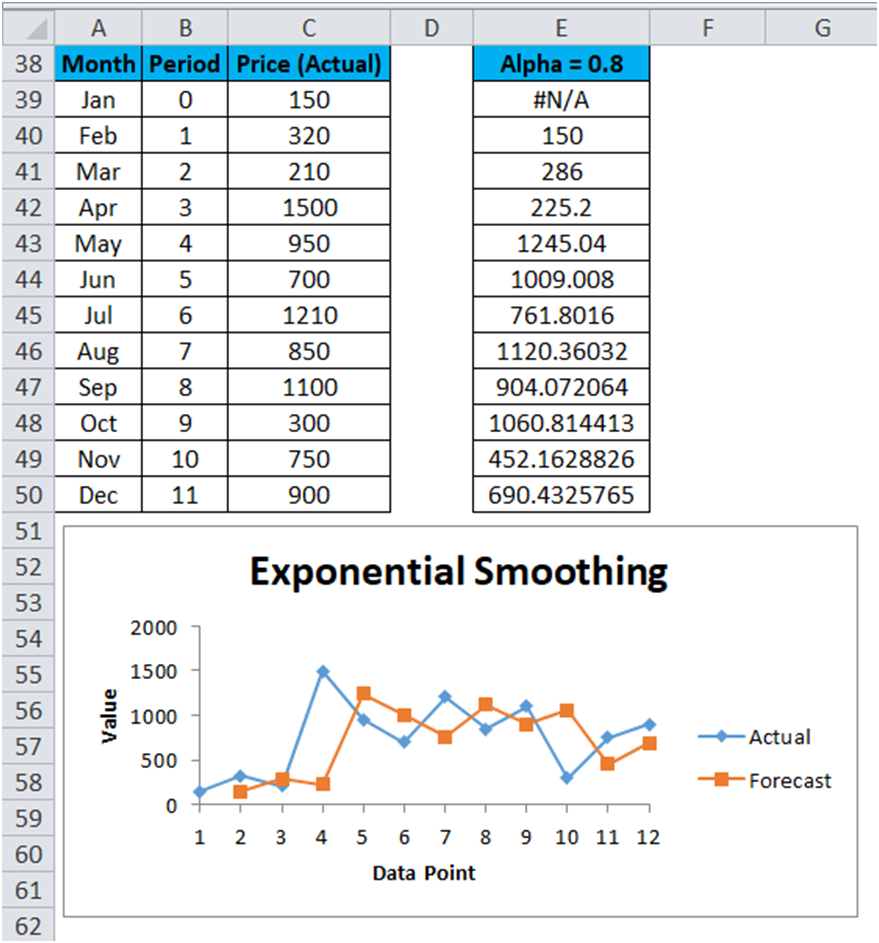
Let’s consider α=0.8 for the above-given data values so enter the value 0.2 in the Damping Factor box and again repeat the Exponential Smoothing method.
The result is shown below:
Now, if we compare the results of all the above 3 Excel Exponential Smoothing examples, then we can come up with the below conclusion:
The Alpha α value is smaller; the damping factor is higher. Resultant the more the peaks and valleys are smoothed out.
The Alpha α value is higher; the damping factor is smaller. Resultant the smoothed values are closer to the actual data points.
Things to Remember
The more value of the dumping factor smooths out the peak and valleys in the dataset.
Excel Exponential Smoothing is a very flexible method to use and easy in the calculation.
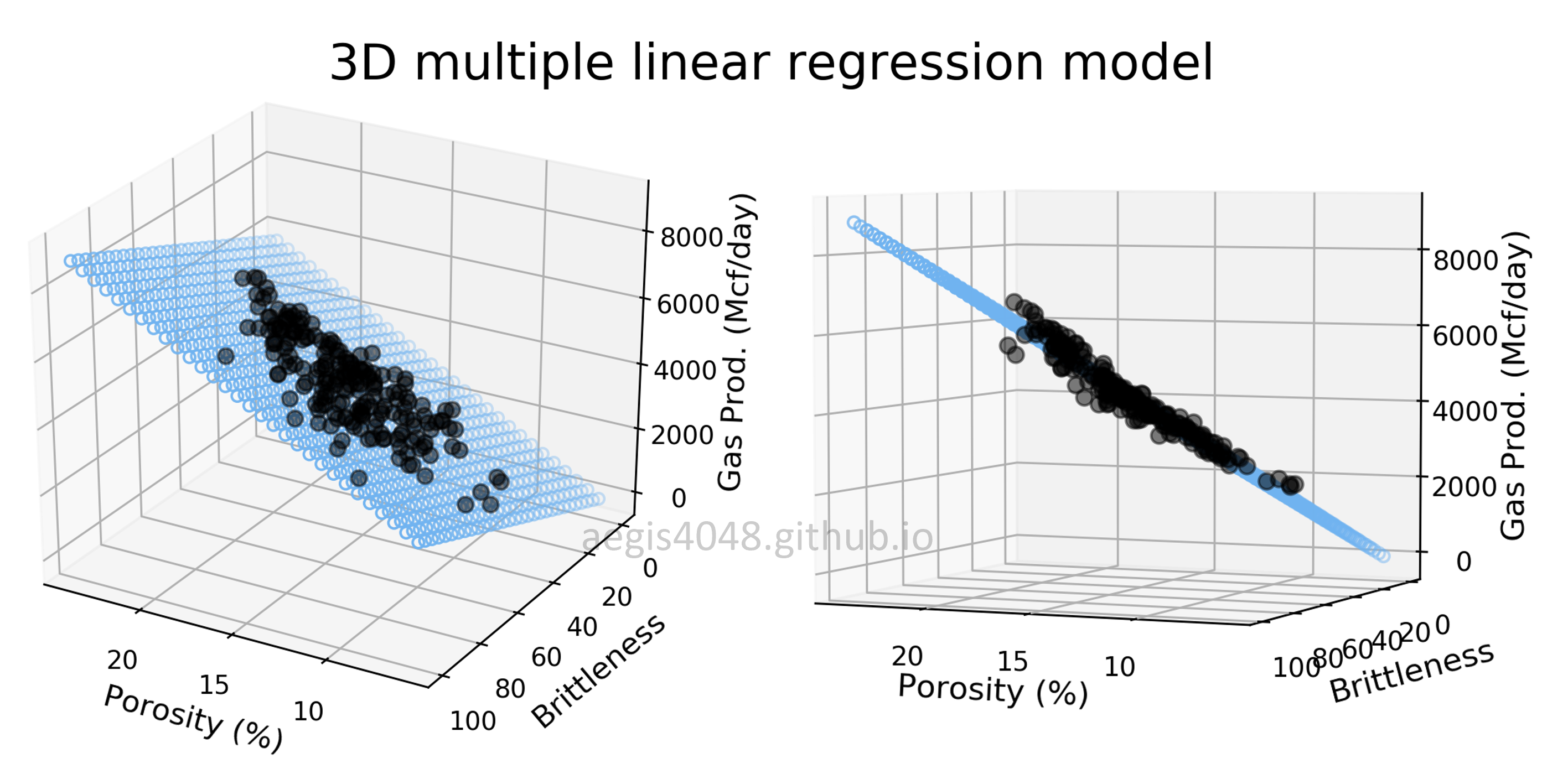
Multiple linear regression (MLR) is a statistical technique that uses several explanatory variables to predict the outcome of a response variable. A linear regression model that contains more than one predictor variable is called a multiple linear regression model. The goal of multiple linear regression (MLR) is to model the relationship between the explanatory and response variables.
The model for MLR, given n observations, is:
Let’s take an example:
The dataset has 5 columns which contains extract from the Profit and Loss statement of 50 start up companies. This tells about the companies R&D, Admin and Marketing spend, the state in which these companies are based and also profit that the companies realized in that year. A venture capitalist (VC) would be interested in such a data and would to see if factors like R&D Spend, Admin expenses, Marketing spend and State has any role to play on the profitability of a startup. This analysis would help VC to make investment decisions in future.
Profit is the dependent variable and other variables are independent variables.
Dummy Variables
Let’s look at the dataset we have for this example:
One challenge we would face while building the linear model is on handling the State variable. State column has a categorical value and can not be treated as like any other numeric value. We need to add dummy variables for each categorical value like below:
Add 3 columns for each categorical value of state. Add 1 to the column where row value of state matches to the column header. Row containing New York will have 1 against the column header New York and rest of the values in that column will be zero. Similarly, we need to modify California and Florida columns too. Three additional columns that we added are called dummy variables and these will be used in our model building. State column can be ignored. We can also ignore New York column from analysis because row which has zero under California and Florida implicitly implies New York will have a value of 1. We always use 1 less dummy variable compared to total factors to avoid dummy variable trap.
Python code:
import pandas as pd import matplotlib.pyplot as plt import numpy as np #Dataset data_df = pd.read_csv(“https://raw.githubusercontent.com/swapnilsaurav/MachineLearning/master/3_Startups.csv”) #Getting X and Y values X = data_df.iloc[:, :-1].values y = data_df.iloc[:, -1].values
#Encoding the categorical variables: from sklearn.preprocessing import LabelEncoder, OneHotEncoder labelencoder_X = LabelEncoder() #Change the text into numbers 0,1,2 – 4th column X[: ,3]= labelencoder_X.fit_transform(X[: ,3]) #create dummy variables from sklearn.compose import ColumnTransformer transformer = ColumnTransformer([(‘one_hot_encoder’, OneHotEncoder(), [3])],remainder=‘passthrough’) #Now a little fit and transform X = np.array(transformer.fit_transform(X), dtype=np.float) #4 Avoid the dummy variables trap #Delete the first column represent the New York X= X[:, 1:]
#Split into training and test set from sklearn.model_selection import train_test_split X_train, X_test, y_train, y_test = train_test_split(X, y, test_size=0.2, random_state=0)
#Train the Algorithm from sklearn.linear_model import LinearRegression regressor = LinearRegression() regressor.fit(X_train, y_train) y_pred = regressor.predict(X_test) #The y_pred is a numpy array that contains all predicted values #compare actual output values for X_test with predicted values output_df = pd.DataFrame({‘Actual’: y_test, ‘Predicted’: y_pred}) print(“Actual v Predicted: \n“,output_df) #### import numpy as np from sklearn import metrics explained_variance=metrics.explained_variance_score(y_test, y_pred) mean_absolute_error=metrics.mean_absolute_error(y_test, y_pred) mse=metrics.mean_squared_error(y_test, y_pred) mean_squared_log_error=metrics.mean_squared_log_error(y_test, y_pred) median_absolute_error=metrics.median_absolute_error(y_test, y_pred) r2=metrics.r2_score(y_test, y_pred) print(‘Explained_variance: ‘, round(explained_variance,2)) print(‘Mean_Squared_Log_Error: ‘, round(mean_squared_log_error,2)) print(‘R-squared: ‘, round(r2,4)) print(‘Mean Absolute Error(MAE): ‘, round(mean_absolute_error,2)) print(‘Mean Squared Error (MSE): ‘, round(mse,2)) print(‘Root Mean Squared Error (RMSE): ‘, round(np.sqrt(mse),2)) from statsmodels.api import OLS import statsmodels.api as sm #In our model, y will be dependent on 2 values: coefficienct # and constant, so we need to add additional column in X for #constant value X = sm.add_constant(X) summ = OLS(y, X).fit().summary() print(“Summary of the dataset: \n“,summ)
Output:
In above table, x1 and x2 are the dummy variables for state, x3 is R&D, x4 is Administration, x5 is the marketing spends.
How many independent variables to consider?
We need to be careful to choose which ones we need to keep for input variables. We do not want to include all the variables for mainly 2 reasons:
GIGO: If we feed garbage to our model we will get garbage out so we need to feed in right set of data
Justifying the input: Can we justify the inclusion of all the data, if no, then we should not include them.
There are 4 methods to build a multiple linear model:
Select all in
Backward Elimination
Forward Selection
Bidirectional Elimination
Select-all-in: We select all the independent variables because we know that all variables impact the result or you have to because business leaders want you to include them.
Backward Elimination:
Select a significance level to stay in the model (e..g. SL =0.05, higher P value to be removed)
Fit the full model with all possible predictors.
Consider the predictor with the highest P-value. If P>SL, go to step 4 otherwise goto 5
Remove the predictor and refit the model and Go to step 3
Your model is ready!
Forward Selection:
Select a significance level to stay in the model (e..g. SL =0.05, lower P value to be kept)
Fit all the simple regression models, Select the one with the lowest P-value.
Keep this variable and fit all possible models with one extra predictor added to the ones you already have. Now Run with 2 variable linear regressions.
Consider the predictor with the lowest P-value. If P<SL, go to Step 3, otherwise go to next step.
Keep the previous model!
Bi-directional Selection: It is a combination of Forward selection and backward elimination:
Select a significant level to enter and stay in the model (SLE = SLS = 0.05)
Perform the next step of Forward selection (new variables must have P<SLE)
Perform all the step of Backward elimination (old variables must have P<SLS)
Iterate between 2 & 3 till no new variables can enter and no old variables can exit.
In the multiple regression example since we have already executed with all the attributes, let’s implement backward elimination method here and remoe out the attributes that are not useful for us. Let’ have a relook at the stats summary:
Look at the highest p-values and remove it. In this condition x2 (second dummy variable has the highest one (0,990). Now, we will remove this variable from the X and re-run the model.
X_opt= X[:, [0,1,3,4,5]] regressor_OLS=sm.OLS(endog = y, exog = X_opt).fit() summ =regressor_OLS.summary() print(“Summary of the dataset after elimination 1: \n“,summ)
Output Snapshot:
Look at the highest p-value again. #First dummy variable, x1’s p-value is 0.940. Remove this one. Even though this appeared as high number in the previous step also, but as per the algorithm we need to remove only 1 value at a time. Since, removing an attribute can have impact on other attributes also. Re-run the code again:
X_opt= X[:, [0,3,4,5]] regressor_OLS=sm.OLS(endog = y, exog = X_opt).fit() summ = regressor_OLS.summary() print(“Summary of the dataset after elimination 2: \n“,summ)
Admin spends (x2) has the highest p-value (0.602). Remove this as well.
X_opt= X[:, [0,3,5]] regressor_OLS=sm.OLS(endog = y, exog = X_opt).fit() summ = regressor_OLS.summary() print(“Summary of the dataset after elimination 3: \n“,summ)
Admin spends (x2) has the highest p-value (0.06). This value is low but since we have selected the significance level (SL) as 0.05, we need to remove this as well.
X_opt= X[:, [0,3]] regressor_OLS=sm.OLS(endog = y, exog = X_opt).fit() summ =regressor_OLS.summary() print(“Summary of the dataset after elimination 3: \n“,summ)
Finally, we see that only one factor has the significant impact on the profit. The highest impact variable is R&D spendings on profit of these startups. The accuracy of the model has also increased. When we included all the attributes, the R squared value was 0.9347 and now its at 0.947.
The word “linear” in “multiple linear regression” refers to the fact that the model meets all the criteria discussed in the next section.
The next question we need to understand is when can we perform or not perform Linear Regression. In this section, let’s understand the assumptions of linear regression in detail. One of the most essential steps to take before applying linear regression and depending solely on accuracy scores is to check for these assumptions and only when a dataset meet these assumptions, we say that dataset can be used for linear regression model.
For the analysis, we will take the same dataset, we used for Multiple Linear Regression Analysis in the previous section.
import pandas as pd #Dataset data_df = pd.read_csv(“https://raw.githubusercontent.com/swapnilsaurav/MachineLearning/master/3_Startups.csv”)
Before we apply regression on all these attributes, we need to understand if we need to really take all of these attributes into consideration. There are two things we need to consider:
First step is to test the dataset if its fits into the linearity definition, which we will perform different tests in this section. Remember, we only test for numerical columns as the categorical columns are not taken into account. As we know that the categorical values are converted into dummy variables of values 0 and 1, dummy variables meet the assumption of linearity by definition, because they creat two data points, and two points define a straight line. There is no such thing as a non-linear relationship for a single variable with only two values.
Code for Prediction: Let’s rewrite the code
import numpy as np X = data_df.iloc[:,:-1].values y = data_df.iloc[:,-1].values
#handling categorical data from sklearn.preprocessing import LabelEncoder, OneHotEncoder le_x = LabelEncoder() X[:,3] = le_x.fit_transform(X[:,3]) from sklearn.compose import ColumnTransformer tranformer = ColumnTransformer([(‘one_hot_encoder’, OneHotEncoder(),[3])], remainder=‘passthrough’) X = np.array(tranformer.fit_transform(X), dtype=np.float) X=X[:,1:]
Linear regression needs the relationship between the independent and dependent variables to be linear. Let’s use a pair plot to check the relation of independent variables with the profit variable.
Output:
Python Code:
import seaborn as sns import matplotlib.pyplot as plt
# visualize the relationship between the features and the response using scatterplots p = sns.pairplot(data_df, x_vars=[‘R&D Spend’,‘Administration’,‘Marketing Spend’], y_vars=‘Profit’, height=5, aspect=0.7) plt.show()
By looking at the plots we can see that with the R&D Spend form an accurately linear shape and Marketing Spend is somewhat in the linear shape but Administration Spend is all over the graph but still shows increasing trend as Profit value increases on Y-Axis. Here we can use Linear Regression models.
2. Variables follow a Normal Distribution
The variables (X) follow a normal distribution. In order words, we want to make sure that for each x value, y is a random variable following a normal distribution and its mean lies on the regression line. One of the ways to visually test for this assumption is through the use of the Q-Q-Plot. Q-Q stands for Quantile-Quantile plot and is a technique to compare two probability distributions in a visual manner. To generate this Q-Q plot we will be using scipy’s probplot function where we compare a variable of our chosen to a normal probability.
import scipy.stats as stats stats.probplot(X[:,3], dist=“norm”, plot=plt) plt.show()
The points must lie on this red line to conclude that it follows a normal distribution. In this case of selecting 3rd column which is R&D Spend, yes it does! A couple of points outside of the line is due to our small sample size. In practice, you decide how strict you want to be as it is a visual test.
3. There is no or littlemulticollinearity
Multicollinearity means that the independent variables are highly correlated with each other. X’s are called independent variables for a reason. If multicollinearity exists between them, they are no longer independent and this generates issues when modeling linear regressions.
To visually test for multicollinearity we can use the power of Pandas. We will use Pandas corr function to compute the pairwise correlation of our columns. If you find any values in which the absolute value of their correlation is >=0.8, the multicollinearity assumption is being broken.
#convert to a pandas dataframe import pandas as pd df = pd.DataFrame(X) df.columns = [‘x1’,‘x2’,‘x3’,‘x4’,‘x5’] #generate correlation matrix corr = df.corr() #Plot HeatMap p=sns.heatmap(df.corr(), annot=True,cmap=‘RdYlGn’,square=True) print(“Corelation Matrix:\n“,corr)
4. Check for Homoscedasticity: The data are needs to be homoscedastic (meaning the residuals are equal across the regression line). Homoscedasticity means that the residuals have equal or almost equal variance across the regression line. By plotting the error terms with predicted terms we can check that there should not be any pattern in the error terms.
#produce regression plots from statsmodels.api import OLS import statsmodels.api as sm X = sm.add_constant(X) model = OLS(y, X).fit() summ = model.summary() print(“Summary of the dataset: \n“,summ) fig = plt.figure(figsize=(12,8)) #Checking for x3 (R&D Spend) fig = sm.graphics.plot_regress_exog(model, ‘x3’, fig=fig) plt.show()
Four plots are produced. The one in the top right corner is the residual vs. fitted plot. The x-axis on this plot shows the actual values for the predictor variable points and the y-axis shows the residual for that value. Since the residuals appear to be randomly scattered around zero, this is an indication that heteroscedasticity is not a problem with the predictor variable x3 (R&D Spend). Multiple Regression, we need to create this plot for each of the predictor variable.
5. Mean of Residuals
Residuals as we know are the differences between the true value and the predicted value. One of the assumptions of linear regression is that the mean of the residuals should be zero. So let’s find out.
residuals = y_test-y_pred mean_residuals = np.mean(residuals) print(“Mean of Residuals {}”.format(mean_residuals))
Output:
Mean of Residuals 3952.010244810798
6. Check for Normality of error terms/residuals
p = sns.distplot(residuals,kde=True) p = plt.title(‘Normality of error terms/residuals’) plt.show()
The residual terms are pretty much normally distributed for the number of test points we took.
A restricted Boltzmann machine (RBM) is a generative stochastic artificial neural network that can learn a probability distribution over its set of inputs. Restricted Boltzmann machines can also be used in deep learning networks. In particular, deep belief networks can be formed by “stacking” RBMs and optionally fine-tuning the resulting deep network with gradient descent and backpropagation. This deep learning algorithm became very popular after the Netflix Competition where RBM was used as a collaborative filtering technique to predict user ratings for movies and beat most of its competition. It is useful for regression, classification, dimensionality reduction, feature learning, topic modelling and collaborative filtering.
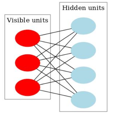
Restricted Boltzmann Machines are stochastic two layered neural networks which belong to a category of energy based models that can detect inherent patterns automatically in the data by reconstructing input. They have two layers visible and hidden. Visible layer has input nodes (nodes which receive input data) and the hidden layer is formed by nodes which extract feature information from the data and the output at the hidden layer is a weighted sum of input layers. They don’t have any output nodes and they don’t have typical binary output through which patterns are learnt. The learning process happens without that capability which makes them different. We only take care of input nodes and don’t worry about hidden nodes. Once the input is provided, RBM’s automatically capture all the patterns, parameters and correlation among the data.
What is Boltzman Machine?
Let’s first undertand what’s Boltzman Machine. Boltzmann Machine was first invented in 1985 by Geoffrey Hinton, a professor at the University of Toronto. He is a leading figure in the deep learning community and is referred to by some as the “Godfather of Deep Learning”.
Boltzman Machine
Boltzmann Machine is a generative unsupervised model, which involves learning a probability distribution from an original dataset and using it to make inferences about never before seen data.
Boltzmann Machine has an input layer (also referred to as the visible layer) and one or several hidden layers (also referred to as the hidden layer).
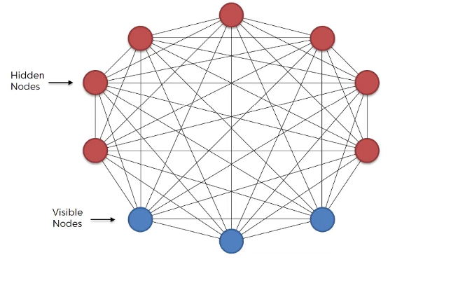
Boltzmann Machine uses neural networks with neurons that are connected not only to other neurons in other layers but also to neurons within the same layer.
Everything is connected to everything. Connections are bidirectional, visible neurons connected to each other and hidden neurons also connected to each other
Boltzmann Machine doesn’t expect input data, it generates data. Neurons generate information regardless they are hidden or visible.
For Boltzmann Machine all neurons are the same, it doesn’t discriminate between hidden and visible neurons. For Boltzmann Machine whole things are system and its generating state of the system.
In Boltzmann Machine, we use our training data and feed into the Boltzmann Machine as input to help the system adjust its weights. It resembles our system not any such system in the world. It learns from the input, what are the possible connections between all these parameters, how do they influence each other and therefore it becomes a machine that represents our system. Boltzmann Machine consists of a neural network with an input layer and one or several hidden layers. The neurons in the neural network make stochastic decisions about whether to turn on or off based on the data we feed during training and the cost function the Boltzmann Machine is trying to minimize. By doing so, the Boltzmann Machine discovers interesting features about the data, which help model the complex underlying relationships and patterns present in the data.
This Boltzmann Machine uses neural networks with neurons that are connected not only to other neurons in other layers but also to neurons within the same layer. That makes training an unrestricted Boltzmann machine very inefficient and Boltzmann Machine had very little commercial success. Boltzmann Machines are primarily divided into two categories: Energy-based Models (EBMs) and Restricted Boltzmann Machines (RBM). When these RBMs are stacked on top of each other, they are known as Deep Belief Networks (DBN). Our focus of discussion here is the RBM.
Restricted Boltzmann Machines (RBM)
Restricted Boltzman Machine Algorithm
What makes RBMs different from Boltzmann machines is that visible node isn’t connected to each other, and hidden nodes aren’t connected with each other. Other than that, RBMs are exactly the same as Boltzmann machines.
It is a probabilistic, unsupervised, generative deep machine learning algorithm.
RBM’s objective is to find the joint probability distribution that maximizes the log-likelihood function.
RBM is undirected and has only two layers, Input layer, and hidden layer
All visible nodes are connected to all the hidden nodes. RBM has two layers, visible layer or input layer and hidden layer so it is also called an asymmetrical bipartite graph.
No intralayer connection exists between the visible nodes. There is also no intralayer connection between the hidden nodes. There are connections only between input and hidden nodes.
The original Boltzmann machine had connections between all the nodes. Since RBM restricts the intralayer connection, it is called a Restricted Boltzmann Machine.
Since RBMs are undirected, they don’t adjust their weights through gradient descent and backpropagation. They adjust their weights through a process called contrastive divergence. At the start of this process, weights for the visible nodes are randomly generated and used to generate the hidden nodes. These hidden nodes then use the same weights to reconstruct visible nodes. The weights used to reconstruct the visible nodes are the same throughout. However, the generated nodes are not the same because they aren’t connected to each other.
Simple Understanding of RBM
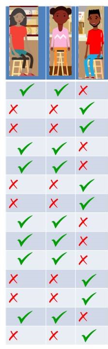
Problem Statement: Let’s take an example of a small café just across a street where people come in the evening to hang out. We see that normally three people: Geeta, Meeta and Paavit visit frequently. Not always all of them show up together. We have all the possible combinations of these three people showing up. It could be just Geeta, Meeta or Paavit show up or Geeta and Meeta come at the same time or Paavit and Meeta or Paavit and Geeta or all three of them show up or none of them show up on some days. All the possibilities are valid.
Left to Right: Geeta, Meeta, Paavit
Let’s say, you watch them coming everyday and make a note of it. Let’s take first day, Meeta and Geeta comes and Paavit didn’t. Second day, Paavit comes but Geeta and Meeta doesn’t. After noticing for 15 days, you find that only these two possibilities are repeated. As represented in the table.
Visits of Geeta, Meeta and Paavit to the cafe
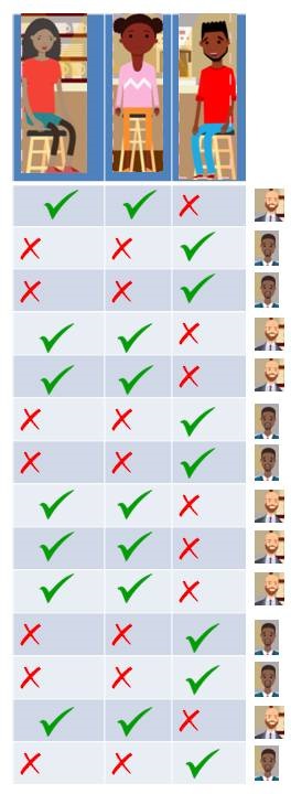
That’s an interesting finding and more so when we come to know that these three people are totally unknown to each other. You also find out that there are two café managers: Ratish and Satish. Lets tabulate it again with 5 people now (3 visitors and 2 managers).
Visits of customer and presence of manager on duty
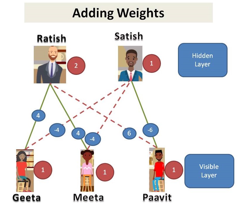
We find that, Geeta and Meeta likes Ratish so they show up when Ratish is on duty. Paavit likes Satish so he shows up only when Satish is on duty. So, we look at the data we might say that Geeta and Meeta went to the café on the days Ratish is on duty and Paavit went when Satish is on duty. Lets add some weights.
Customers and Managers relation with weights
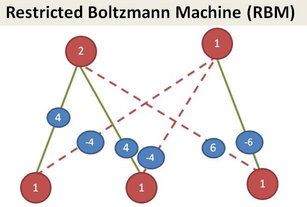
Since we see that customers in our dataset, we call them as visible layer. Managers are not shown in the dataset, we call it as hidden layer. This is an example of Restricted Boltzmann Machine (RBM).
RBM
(… to be continued…)
Working of RBM
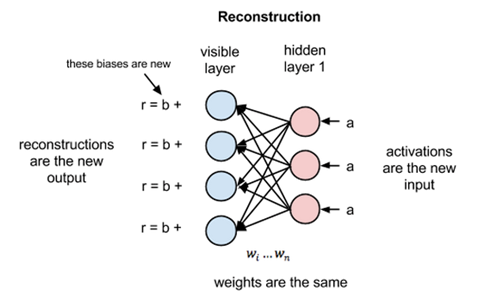
RBM is a Stochastic Neural Network which means that each neuron will have some random behavior when activated. There are two other layers of bias units (hidden bias and visible bias) in an RBM. This is what makes RBMs different from autoencoders. The hidden bias RBM produces the activation on the forward pass and the visible bias helps RBM to reconstruct the input during a backward pass. The reconstructed input is always different from the actual input as there are no connections among the visible units and therefore, no way of transferring information among themselves.
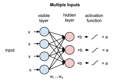
Step 1
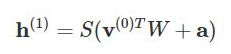
The above image shows the first step in training an RBM with multiple inputs. The inputs are multiplied by the weights and then added to the bias. The result is then passed through a sigmoid activation function and the output determines if the hidden state gets activated or not. Weights will be a matrix with the number of input nodes as the number of rows and the number of hidden nodes as the number of columns. The first hidden node will receive the vector multiplication of the inputs multiplied by the first column of weights before the corresponding bias term is added to it.
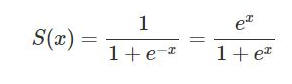
Here is the formula of the Sigmoid function shown in the picture:
So the equation that we get in this step would be,
where h(1) and v(0) are the corresponding vectors (column matrices) for the hidden and the visible layers with the superscript as the iteration v(0) means the input that we provide to the network) and a is the hidden layer bias vector.
(Note that we are dealing with vectors and matrices here and not one-dimensional values.)
Now this image shows the reverse phase or the reconstruction phase. It is similar to the first pass but in the opposite direction. The equation comes out to be:
where v(1) and h(1) are the corresponding vectors (column matrices) for the visible and the hidden layers with the superscript as the iteration and b is the visible layer bias vector.
Now, the difference v(0)−v(1) can be considered as the reconstruction error that we need to reduce in subsequent steps of the training process. So the weights are adjusted in each iteration so as to minimize this error and this is what the learning process essentially is.
In the forward pass, we are calculating the probability of output h(1) given the input v(0) and the weights W denoted by:
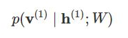
And in the backward pass, while reconstructing the input, we are calculating the probability of output v(1) given the input h(1) and the weights W denoted by:
The weights used in both the forward and the backward pass are the same. Together, these two conditional probabilities lead us to the joint distribution of inputs and the activations:
Reconstruction is different from regression or classification in that it estimates the probability distribution of the original input instead of associating a continuous/discrete value to an input example. This means it is trying to guess multiple values at the same time. This is known as generative learning as opposed to discriminative learning that happens in a classification problem (mapping input to labels).
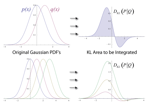
Let us try to see how the algorithm reduces loss or simply put, how it reduces the error at each step. Assume that we have two normal distributions, one from the input data (denoted by p(x)) and one from the reconstructed input approximation (denoted by q(x)). The difference between these two distributions is our error in the graphical sense and our goal is to minimize it, i.e., bring the graphs as close as possible. This idea is represented by a term called the Kullback–Leibler divergence.
KL-divergence measures the non-overlapping areas under the two graphs and the RBM’s optimization algorithm tries to minimize this difference by changing the weights so that the reconstruction closely resembles the input. The graphs on the right-hand side show the integration of the difference in the areas of the curves on the left.
This gives us intuition about our error term. Now, to see how actually this is done for RBMs, we will have to dive into how the loss is being computed. All common training algorithms for RBMs approximate the log-likelihood gradient given some data and perform gradient ascent on these approximations.
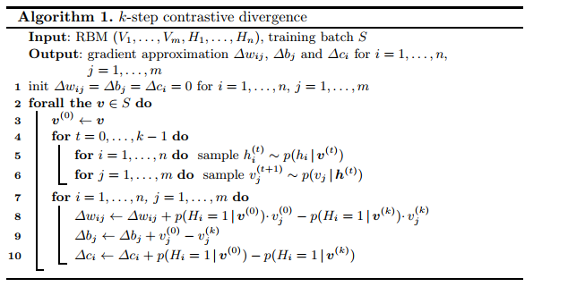
Contrastive Divergence
Here is the pseudo-code for the CD algorithm:
CD Algorithm pseudo code
Applications: * Pattern recognition : RBM is used for feature extraction in pattern recognition problems where the challenge is to understand the hand written text or a random pattern. * Recommendation Engines : RBM is widely used for collaborating filtering techniques where it is used to predict what should be recommended to the end user so that the user enjoys using a particular application or platform. For example : Movie Recommendation, Book Recommendation * Radar Target Recognition : Here, RBM is used to detect intra pulse in Radar systems which have very low SNR and high noise.
Source: wikipedia (https://en.wikipedia.org/wiki/Restricted_Boltzmann_machine)
The RStudio IDE is a set of integrated tools designed to help you be more productive with R and Python. It includes a console, syntax-highlighting editor that supports direct code execution, and a variety of robust tools for plotting, viewing history, debugging and managing your workspace.
If you want to start practicing r programs then R Studio is the best IDE. In this section, I will write the steps on how you can install RStudio Desktop for your personal use. RStudio Desktop is totally free to use.
Click the “download R” link in the middle of the page under “Getting Started.”
Select a CRAN location (a mirror site) and click the corresponding link.
Click on the “Download R for Windows” link at the top of the page.
Click on the “install R for the first time” link at the top of the page.
Click “Download R for Windows” and save the executable file somewhere on your computer. Run the .exe file and follow the installation instructions.
Now that R is installed, you need to download and install RStudio.
To Install RStudio
Go to www.rstudio.com and click on the “Download RStudio” button.
Click on “Download RStudio Desktop.”
Click on the version recommended for your system, or the latest Windows version, and save the executable file. Run the .exe file and follow the installation instructions.
I hope you have installed R and R studio and now you are ready to practice your programs.
If you are unsure about any setting, accept the defaults. You can change them later.
When installation is finished, from the Start menu, open the Anaconda Prompt.
Test your installation. In your terminal window or Anaconda Prompt, run the command condalist. A list of installed packages appears if it has been installed correctly.